Cholesky, log-det, trace — the structured primitives tour

Every Gaussian computation in this curriculum eventually bottoms out into one of four scalar/array reductions of a covariance / precision operator $A$ :

Primitive	What it returns	Where it shows up
`cholesky(A)`	factor $L$ s.t. $A = L L^\top$	sampling, log-density, conditioning
`logdet(A)`	$\log\lvert A\rvert$	log-density, marginal likelihood, KL, entropy
`trace(A)`	$\sum_i A_{ii}$	KL, ELBO, expected log-likelihood, score test
`diag(A)`	$(A_{11},\dots,A_{nn})$	predictive marginal variance, calibration

In gaussx these are structurally dispatched: hand them a DiagonalLinearOperator and you get an $\mathcal{O}(n)$ closed-form; hand them a Kronecker(A,B) and they exploit $\det(A\otimes B) = \det(A)^{n_B}\det(B)^{n_A}$ ; everything else falls back to dense Cholesky-via-LAPACK. The dispatch is invisible to the caller — this notebook makes it visible.

This is not a list of identities — those live in 0.3 — quadratic forms, entropy, KL. It’s the operational layer underneath: which structures get cheap special-cases, what the cost is, and how the dispatch composes with the operator zoo from 0.8 — structured sampling.

Prerequisites: 0.1 — multivariate Gaussian, 0.3 — Gaussian quantities, 0.8 — structured sampling.

from __future__ import annotations

import warnings
warnings.filterwarnings("ignore", message=r".*IProgress.*")

import time
import einx
import jax
import jax.numpy as jnp
import lineax as lx
import matplotlib.pyplot as plt
import numpy as np
from gaussx import (
    BlockDiag, BlockTriDiag, Kronecker,
    cholesky, diag as gx_diag, logdet, trace as gx_trace,
)

jax.config.update("jax_enable_x64", True)
KEY = jax.random.PRNGKey(0)
plt.rcParams.update({
    "figure.dpi": 110,
    "axes.grid": True,
    "axes.grid.which": "both",
    "xtick.minor.visible": True,
    "ytick.minor.visible": True,
    "grid.alpha": 0.3,
})

def psd_op(M):
    return lx.MatrixLinearOperator(M, lx.positive_semidefinite_tag)

def random_psd(key, n, jitter=1e-3):
    A = jax.random.normal(key, (n, n))
    return A @ A.T + jitter * jnp.eye(n)

The four primitives — what they compute¶

For a symmetric positive-definite (SPD) matrix $A \in \mathbb{R}^{n \times n}$ , the Cholesky factorisation is the unique lower-triangular matrix $L$ with positive diagonal such that

A \;=\; L L^\top.

((1))

Every other primitive in this section can be derived from $L$ :

\log\lvert A \rvert \;=\; \log\bigl\lvert L L^\top \bigr\rvert \;=\; 2\sum_{i=1}^{n} \log L_{ii}.

((2))

A_{ii} \;=\; \sum_{k=1}^{i} L_{ik}^{2}, \qquad \mathrm{tr}(A) \;=\; \sum_{i,k} L_{ik}^{2} \;=\; \lVert L \rVert_F^2.

((3))

((2)) is the workhorse: $\log\lvert A\rvert$ never needs to materialise the full determinant — overflow / underflow is impossible because we sum logs of $n$ positive scalars. ((3)) shows that the diagonal of $A$ and its trace are both quadratic forms in the rows of $L$ .

Dispatch — closed-form identities, compute, storage¶

The four primitives dispatch on operator type. To keep the picture honest we separate three orthogonal questions:

Which closed-form identity is used? (the math)
What does it cost to compute? (FLOPs / time)
What does the operator and its factor occupy in memory? (storage)

All three matter — a structure can have a cheap closed-form but bad storage (densified factor), or vice versa. The tables below cover the four operator types with full primitive coverage in gaussx today: Diagonal, Kronecker, BlockDiag, BlockTriDiag. (LowRankUpdate has dispatched logdet via the determinant lemma but no closed-form cholesky — it appears in 0.8 — structured sampling.)

1. Closed-form identities¶

Operator	`cholesky(A)`	`logdet(A)`	`trace(A)`	`diag(A)`
`Diagonal(d)`	$\mathrm{diag}(\sqrt{d})$	$\sum_i \log d_i$	$\sum_i d_i$	$d$
`Kronecker(A,B)`	$L_A \otimes L_B$	$n_B\log\lvert A\rvert + n_A\log\lvert B\rvert$	$\mathrm{tr}(A)\,\mathrm{tr}(B)$	$\mathrm{diag}(A)\otimes\mathrm{diag}(B)$
`BlockDiag([A_k])`	$\mathrm{BlockDiag}(L_{A_k})$	$\sum_k \log\lvert A_k\rvert$	$\sum_k \mathrm{tr}(A_k)$	$\mathrm{concat}(\mathrm{diag}(A_k))$
`BlockTriDiag`	banded $L$ (`LowerBlockTriDiag`)	$2\sum_i \log L_{ii}$	$\sum_k \mathrm{tr}(D_k)$	per-block $\mathrm{diag}(D_k)$
dense fallback	LAPACK Cholesky	$2\sum_i \log L_{ii}$	$\sum_i A_{ii}$	$A_{ii}$

Each row is an exact algebraic identity — not an approximation. The structured Cholesky returns the same operator type (Kronecker stays Kronecker, BlockDiag stays BlockDiag), so downstream solve / mv keep their structure too.

2. Compute cost (asymptotic FLOPs)¶

Total size $n =$ leading dimension of $A$ . For Kronecker we set $n = n_A n_B$ ; for BlockDiag with $K$ blocks of size $b$ , $n = Kb$ ; for BlockTriDiag with $N$ blocks of size $b$ , $n = Nb$ .

Operator	`cholesky`	`logdet`	`trace`	`diag`
`Diagonal(d)`	$\mathcal{O}(n)$	$\mathcal{O}(n)$	$\mathcal{O}(n)$	$\mathcal{O}(n)$
`Kronecker(A,B)`	$\mathcal{O}(n_A^3 + n_B^3)$	$\mathcal{O}(n_A^3 + n_B^3)$	$\mathcal{O}(n_A + n_B)$	$\mathcal{O}(n_A + n_B)$
`BlockDiag`, $K$ blocks of size $b$	$\mathcal{O}(K b^3)$	$\mathcal{O}(K b^3)$	$\mathcal{O}(K b)$	$\mathcal{O}(K b)$
`BlockTriDiag`, $N$ blocks of size $b$	$\mathcal{O}(N b^3)$	$\mathcal{O}(N b^3)$	$\mathcal{O}(N b)$	$\mathcal{O}(N b)$
dense fallback	$\mathcal{O}(n^3)$	$\mathcal{O}(n^3)$	$\mathcal{O}(n)$	$\mathcal{O}(n)$

The big wins are cholesky and logdet — sub-cubic scaling in the structured rows. A $100\times 100$ Kronecker of two $10\times 10$ factors needs $\mathcal{O}(2\cdot 10^3)$ FLOPs vs $\mathcal{O}(100^3) = 500\times$ larger for the dense path.

3. Storage cost¶

Operator	operator $A$	Cholesky factor $L$
`Diagonal(d)`	$\mathcal{O}(n)$	$\mathcal{O}(n)$
`Kronecker(A,B)`	$\mathcal{O}(n_A^2 + n_B^2)$	$\mathcal{O}(n_A^2 + n_B^2)$ — stays `Kronecker`
`BlockDiag`, $K$ blocks of size $b$	$\mathcal{O}(K b^2)$	$\mathcal{O}(K b^2)$ — stays `BlockDiag`
`BlockTriDiag`, $N$ blocks of size $b$	$\mathcal{O}(N b^2)$	$\mathcal{O}(N b^2)$ — banded `LowerBlockTriDiag`
dense fallback	$\mathcal{O}(n^2)$	$\mathcal{O}(n^2)$

The row that matters most: the Cholesky factor inherits the operator’s storage class. If cholesky(Kronecker(A,B)) densified the factor, you’d pay $\mathcal{O}((n_A n_B)^2)$ memory — defeating the purpose. gaussx keeps the factor in the same class, so memory + downstream solve / mv cost both stay sub-quadratic.

A side-by-side: dense vs structured¶

We build the same SPD matrix in two ways — once as a generic MatrixLinearOperator (dense), once as a Kronecker — and confirm:

all four primitives return the same numerical answer;
the structured path goes through closed-form code (verifiable by inspecting the dispatched function names, not just timing).

# Build A = K_A ⊗ K_B as both a Kronecker operator and a dense MatrixLinearOperator.
key1, key2 = jax.random.split(KEY)
n_A, n_B = 8, 6
K_A_dense = random_psd(key1, n_A, jitter=0.5)
K_B_dense = random_psd(key2, n_B, jitter=0.5)
K_A_op = psd_op(K_A_dense)
K_B_op = psd_op(K_B_dense)

A_kron = Kronecker(K_A_op, K_B_op)         # structured operator — n_A * n_B = 48
A_dense = psd_op(A_kron.as_matrix())       # same matrix, no structural tag

print(f"shape:                 {A_kron.in_size()} x {A_kron.in_size()}")
print(f"||A_kron - A_dense||F: {float(jnp.linalg.norm(A_kron.as_matrix() - A_dense.as_matrix())):.3e}")

shape:                 48 x 48
||A_kron - A_dense||F: 0.000e+00

# Compare all four primitives — structured vs dense.
def report(name, val_struct, val_dense, atol=1e-9):
    err = float(jnp.linalg.norm(jnp.asarray(val_struct) - jnp.asarray(val_dense)))
    flag = "OK" if err < atol else "MISMATCH"
    print(f"  {name:<10}  struct vs dense ||·||  =  {err:.3e}   [{flag}]")

L_kron = cholesky(A_kron)         # returns a Kronecker(L_A, L_B)
L_dense = cholesky(A_dense)        # returns a TriangularLinearOperator (lower)

print(f"cholesky type (struct): {type(L_kron).__name__}")
print(f"cholesky type (dense):  {type(L_dense).__name__}")
print()
report("cholesky", L_kron.as_matrix(), L_dense.as_matrix())
report("logdet",   logdet(A_kron),    logdet(A_dense))
report("trace",    gx_trace(A_kron),  gx_trace(A_dense))
report("diag",     gx_diag(A_kron),   gx_diag(A_dense))

cholesky type (struct): Kronecker
cholesky type (dense):  MatrixLinearOperator

  cholesky    struct vs dense ||·||  =  2.357e-14   [OK]

  logdet      struct vs dense ||·||  =  2.842e-14   [OK]

  trace       struct vs dense ||·||  =  0.000e+00   [OK]

  diag        struct vs dense ||·||  =  0.000e+00   [OK]

The structured Cholesky returns a Kronecker operator. That’s the entire point — the factor itself stays structured, so subsequent solve / mv calls also remain $\mathcal{O}(n_A^3 + n_B^3)$ rather than $\mathcal{O}((n_A n_B)^3)$ . The dense path returns a triangular operator with a full $n \times n$ matrix.

The numerical results agree to working precision — all four primitives give the same answer regardless of which dispatch fires. The cost difference is what changes.

Where each primitive shows up¶

A quick map from primitives to the Gaussian quantities you’ll see in the rest of Part 0–1:

\log\mathcal{N}(x \mid \mu, \Sigma) \;=\; -\tfrac{1}{2}\,\underbrace{(x-\mu)^\top \Sigma^{-1}(x-\mu)}_{\text{quadratic form via }L} \;-\; \tfrac{1}{2}\,\underbrace{\log\lvert \Sigma\rvert}_{\texttt{logdet}} \;-\; \tfrac{n}{2}\log(2\pi).

((4))

\mathrm{KL}\bigl(\mathcal{N}(\mu_0,\Sigma_0) \,\|\, \mathcal{N}(\mu_1,\Sigma_1)\bigr) \;=\; \tfrac{1}{2}\bigl[\,\underbrace{\mathrm{tr}(\Sigma_1^{-1}\Sigma_0)}_{\texttt{trace}} \;+\; \underbrace{(\mu_1-\mu_0)^\top \Sigma_1^{-1}(\mu_1-\mu_0)}_{\text{solve}} \;-\; n \;+\; \underbrace{\log\lvert\Sigma_1\rvert - \log\lvert\Sigma_0\rvert}_{\texttt{logdet}}\,\bigr].

((5))

\mathbb{H}\bigl[\mathcal{N}(\mu,\Sigma)\bigr] \;=\; \tfrac{n}{2}\bigl(1 + \log(2\pi)\bigr) \;+\; \tfrac{1}{2}\,\underbrace{\log\lvert\Sigma\rvert}_{\texttt{logdet}}.

((6))

\sigma_{\star,i}^{2} \;=\; \bigl[\mathrm{diag}(K_{\star\star} - K_{\star X} K_{XX}^{-1} K_{X\star})\bigr]_{i} \;\Longrightarrow\; \texttt{diag} \;\circ\; \texttt{cov\_transform}.

((7))

((4)) is the standard Gaussian log-density; ((5)) the KL between two Gaussians (compare with ); ((6)) the differential entropy; ((7)) the predictive marginal variance you’ll see throughout part 3 / 5. Every Gaussian quantity is a small expression in the four primitives.

Asymptotic cost — straight from the table¶

Rather than benchmark each combination empirically (which is noisy and machine-dependent), we plot the theoretical FLOP counts from the dispatch table directly. The shapes of the curves are what matter — they tell you which structures pay off as $n$ grows.

For an operator of total size $n$ , we count one constant per leading-order term and sweep $n \in [4, 4096]$ .

Diagonal: every primitive is $\mathcal{O}(n)$ .
Kronecker(n_A, n_B) with $n_A = n_B = \sqrt{n}$ : chol/logdet are $\mathcal{O}(n^{3/2})$ , trace/diag are $\mathcal{O}(\sqrt{n})$ .
BlockDiag / BlockTriDiag with fixed block size $b = 8$ : chol/logdet are $\mathcal{O}(n)$ (linear in number-of-blocks × $b^3$ constant).
dense fallback: chol/logdet are $\mathcal{O}(n^3)$ , trace/diag are $\mathcal{O}(n)$ .

# Theoretical FLOP counts straight from the dispatch table.
# n is the total leading dimension; each operator has its parameters set so its size is n.
b = 8                                                # block size for BlockDiag / BlockTriDiag
ns = np.logspace(np.log10(16), np.log10(4096), 60)   # log-spaced sweep

# {primitive: {operator: flops(n)}}
flops = {
    "cholesky / logdet": {
        "Diagonal":     ns,                          # O(n)
        "Kronecker":    2 * ns**1.5,                 # O(n_A^3 + n_B^3) with n_A=n_B=sqrt(n)
        "BlockDiag":    (ns / b) * b**3,             # K=n/b blocks, b^3 each
        "BlockTriDiag": (ns / b) * b**3,             # same leading order
        "dense":        ns**3,                       # O(n^3)
    },
    "trace / diag": {
        "Diagonal":     ns,                          # O(n)
        "Kronecker":    2 * np.sqrt(ns),             # O(n_A + n_B)
        "BlockDiag":    ns,                          # K * b = n
        "BlockTriDiag": ns,                          # N * b = n
        "dense":        ns,                          # O(n)
    },
}

colors = {"Diagonal": "tab:purple", "Kronecker": "forestgreen",
          "BlockDiag": "steelblue", "BlockTriDiag": "darkorange",
          "dense": "crimson"}

fig, axes = plt.subplots(1, 2, figsize=(11.5, 4.4), sharex=True)
for ax, (title, curves) in zip(axes, flops.items()):
    for op, y in curves.items():
        ls = "--" if op == "dense" else "-"
        ax.plot(ns, y, ls, lw=1.8, color=colors[op], label=op)
    ax.set_xscale("log"); ax.set_yscale("log")
    ax.set_xlabel(r"matrix size  $n$")
    ax.set_ylabel("FLOPs (leading order, arbitrary units)")
    ax.set_title(title)
    ax.legend(frameon=False, fontsize=9, loc="upper left")

plt.tight_layout(); plt.show()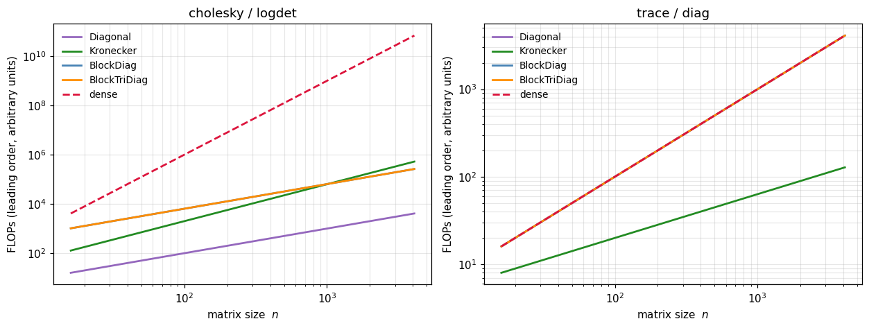

Left panel — cholesky / logdet. The dense curve climbs at $\mathcal{O}(n^3)$ ; the structured curves bend down sharply: Kronecker at $\mathcal{O}(n^{3/2})$ , BlockDiag and BlockTriDiag at $\mathcal{O}(n)$ (for fixed block size), Diagonal also $\mathcal{O}(n)$ . By $n = 4096$ the gap between dense and Kronecker is over four orders of magnitude.

Right panel — trace / diag. All operators land at $\mathcal{O}(n)$ or below; Kronecker even drops to $\mathcal{O}(\sqrt{n})$ because $\mathrm{tr}(A\otimes B) = \mathrm{tr}(A)\,\mathrm{tr}(B)$ only touches each factor’s diagonal. These operations are cheap regardless — the win there is storage (you never materialise $A$ ), not flops.

This is the same conclusion we reached in 0.8 — structured sampling for cholesky-via-mv: the structure-preserving primitive gives you sub-cubic scaling without writing any custom code. You just instantiate the right operator type, and gaussx routes through the closed-form path automatically.

BlockDiag — independent components¶

Block-diagonal covariances arise whenever you have independent Gaussian sub-models — independent outputs in a multi-task GP, independent particles in an ensemble, independent agents in a multi-agent state-space. The dispatch acts on each block in parallel.

\log\bigl\lvert\,\mathrm{diag}(A_1,\dots,A_K)\,\bigr\rvert \;=\; \sum_{k=1}^{K} \log\lvert A_k\rvert.

((8))

# BlockDiag of three SPD blocks of differing sizes.
keys = jax.random.split(jax.random.PRNGKey(11), 3)
blocks = [psd_op(random_psd(k, n, jitter=0.5)) for k, n in zip(keys, [4, 6, 5])]
A_bd = BlockDiag(*blocks)
A_de = psd_op(A_bd.as_matrix())

print(f"shape:                {A_bd.in_size()} x {A_bd.in_size()}")
print(f"cholesky type:        {type(cholesky(A_bd)).__name__}    (preserves block structure)")
print(f"logdet  struct/dense:  {float(logdet(A_bd)):>+.6f}  /  {float(logdet(A_de)):>+.6f}")
print(f"trace   struct/dense:  {float(gx_trace(A_bd)):>+.6f}  /  {float(gx_trace(A_de)):>+.6f}")
print(f"diag    ||struct - dense||: {float(jnp.linalg.norm(gx_diag(A_bd) - gx_diag(A_de))):.3e}")

shape:                15 x 15
cholesky type:        BlockDiag    (preserves block structure)

logdet  struct/dense:  +18.042260  /  +18.042260
trace   struct/dense:  +92.189598  /  +92.189598

diag    ||struct - dense||: 0.000e+00

The Cholesky of a BlockDiag is a BlockDiag — same structure-preserving idea as Kronecker. The $K$ blocks are factored independently (and in parallel under JIT), so the cost scales linearly in the number of blocks rather than cubically in their total size.

Diagonal — the trivial case¶

The cheapest covariance is a diagonal one. All four primitives reduce to elementwise ops on the diagonal vector $d$ :

\mathrm{cholesky}(\mathrm{diag}(d)) = \mathrm{diag}(\sqrt{d}), \quad \log\lvert \mathrm{diag}(d)\rvert = \sum_i \log d_i, \quad \mathrm{tr}(\mathrm{diag}(d)) = \sum_i d_i, \quad \mathrm{diag}(\mathrm{diag}(d)) = d.

((9))

This isn’t just a curiosity — diagonal noise covariances $R = \sigma^2 I$ are the Gaussian assumption in observation models, and the per-output noise diagonals show up in heteroscedastic GPs (part 3.C).

# Diagonal operator — closed-form everything.
d = jnp.array([2.0, 0.5, 1.5, 0.1])
D = lx.DiagonalLinearOperator(d)

print(f"cholesky:  {jnp.asarray(cholesky(D).as_matrix()).diagonal()}        (= sqrt(d))")
print(f"logdet:    {float(logdet(D)):+.6f}             (= sum(log d))")
print(f"trace:     {float(gx_trace(D)):+.6f}             (= sum d)")
print(f"diag:      {jnp.asarray(gx_diag(D))}        (= d)")

cholesky:  [1.41421356 0.70710678 1.22474487 0.31622777]        (= sqrt(d))

logdet:    -1.897120             (= sum(log d))
trace:     +4.100000             (= sum d)
diag:      [2.  0.5 1.5 0.1]        (= d)

Stochastic estimation — when even diag/trace are too expensive¶

For very large $A$ (e.g. an implicit kernel operator at scale, or the Hessian of a deep network), even the $\mathcal{O}(n)$ diagonal extraction is too costly when $A$ itself isn’t materialised. gaussx supports Hutchinson-style stochastic estimators for trace and diag:

\mathrm{tr}(A) \;=\; \mathbb{E}_{\varepsilon}\bigl[\,\varepsilon^\top A\,\varepsilon\,\bigr], \qquad \varepsilon_i \in \{\pm 1\} \text{ Rademacher}.

((10))

\mathrm{diag}(A)_i \;\approx\; \frac{1}{N}\sum_{k=1}^{N} \varepsilon_i^{(k)} \,(A\varepsilon^{(k)})_i, \qquad \varepsilon^{(k)} \sim \{\pm 1\}^n.

((11))

((10)) is exact in expectation and uses only matvecs with $A$ — no factorisation. ((11)) is the Bekas–Kokiopoulou–Saad probing estimator for the diagonal. Both are critical for the BBMM / Lanczos / SLQ stack in part 1.E.

# Hutchinson stochastic trace via gaussx.trace's `n_samples=` argument.
key_st = jax.random.PRNGKey(123)
n_big = 64
A_big = psd_op(random_psd(jax.random.PRNGKey(99), n_big, jitter=1.0))

tr_exact = float(gx_trace(A_big))
tr_stoch_64  = float(gx_trace(A_big, stochastic=True, key=key_st, num_probes=64))
tr_stoch_256 = float(gx_trace(A_big, stochastic=True, key=key_st, num_probes=256))
tr_stoch_2k  = float(gx_trace(A_big, stochastic=True, key=key_st, num_probes=2048))

print(f"exact trace               : {tr_exact:>10.4f}")
print(f"stochastic trace (N=64)   : {tr_stoch_64:>10.4f}    rel. err {abs(tr_stoch_64-tr_exact)/abs(tr_exact):.3%}")
print(f"stochastic trace (N=256)  : {tr_stoch_256:>10.4f}    rel. err {abs(tr_stoch_256-tr_exact)/abs(tr_exact):.3%}")
print(f"stochastic trace (N=2048) : {tr_stoch_2k:>10.4f}    rel. err {abs(tr_stoch_2k-tr_exact)/abs(tr_exact):.3%}")

exact trace               :  4232.2136
stochastic trace (N=64)   :  4245.3880    rel. err 0.311%
stochastic trace (N=256)  :  4201.2455    rel. err 0.732%
stochastic trace (N=2048) :  4229.7748    rel. err 0.058%

The estimator’s variance scales as $\mathcal{O}(1/N)$ , so the relative error halves when you 4× the sample budget. For applications that only need an unbiased gradient estimate (e.g. log-determinant gradients via stochastic Lanczos quadrature, or score-function estimators of marginal likelihood), this is more than enough — you take a noisy estimate and let SGD average it out.

Recap¶

Four primitives — cholesky, logdet, trace, diag — power every Gaussian quantity in the curriculum: log-density ((4)), KL ((5)), entropy ((6)), predictive marginals ((7)).
All four dispatch structurally in gaussx: Diagonal / BlockDiag / Kronecker / BlockTriDiag / LowRankUpdate get closed-form $\mathcal{O}(n)$ – $\mathcal{O}(n^{3/2})$ paths; everything else falls back to dense LAPACK.
The Cholesky of a structured operator is itself a structured operator — cholesky(Kronecker(A,B)) = Kronecker(L_A, L_B) — so downstream solve / mv calls stay sub-cubic.
Hutchinson / Bekas–Kokiopoulou stochastic estimators provide $\mathcal{O}(1/N)$ unbiased estimates of trace and diag for matrix-free operators where even $\mathcal{O}(n)$ extraction is too expensive — the entry point to BBMM-style scaling.