Quadratic forms, entropy, KL — closed-form Gaussian quantities

Why is variational inference with Gaussian distributions so much faster than VI with anything else? Because every quantity you need — log-density, entropy, score, KL, expected log-likelihood, mutual information — has a closed form in terms of $\boldsymbol{\mu}$ , $\boldsymbol{\Sigma}$ , and a Cholesky factor. No Monte Carlo, no quadrature, just linear algebra. This notebook is the catalog.

What you’ll learn

The quadratic form $\tfrac{1}{2}(\mathbf{x}-\boldsymbol{\mu})^\top\boldsymbol{\Sigma}^{-1}(\mathbf{x}-\boldsymbol{\mu})$ — the workhorse, computed via Cholesky and triangular solves.
Score $\nabla_{\mathbf{x}}\log p(\mathbf{x})$ — fundamental for HMC, Langevin, diffusion, score matching.
Entropy and cross-entropy, and the identity that links them to KL.
KL between two Gaussians — full closed form, asymmetry, mode-covering vs mode-seeking.
Expected log-likelihood under a Gaussian — the data-fit term of every Gaussian ELBO.
Mutual information between sub-blocks — closed-form information geometry of an MVN.
A one-step ELBO putting the closed-form KL and ELL together.

from __future__ import annotations

import warnings

warnings.filterwarnings("ignore", message=r".*IProgress.*")

import einx
import jax
import jax.numpy as jnp
import lineax as lx
import matplotlib.pyplot as plt
import numpy as np
from gaussx import (
    MultivariateNormal,
    add_jitter,
    cholesky,
    dist_kl_divergence,
    gaussian_entropy,
    gaussian_expected_log_lik,
    gaussian_log_prob,
    kl_standard_normal,
    quadratic_form,
    solve,
)

jax.config.update("jax_enable_x64", True)
KEY = jax.random.PRNGKey(0)
plt.rcParams.update({
    "figure.dpi": 110,
    "axes.grid": True,
    "axes.grid.which": "both",
    "xtick.minor.visible": True,
    "ytick.minor.visible": True,
    "grid.alpha": 0.3,
})

def psd_op(M):
    return lx.MatrixLinearOperator(M, lx.positive_semidefinite_tag)

1. The quadratic form $\delta^\top \boldsymbol{\Sigma}^{-1}\delta$ ¶

What it is. The bilinear form below is the squared Mahalanobis distance from $\mathbf{x}$ to the mean. Geometrically it’s the squared Euclidean distance after whitening — i.e. after rotating and rescaling so that $\boldsymbol{\Sigma}$ looks like the identity. So contours of constant $Q$ are exactly the Mahalanobis ellipsoids of 0.1 §2.

Continuous form.

Q(\mathbf{x}; \boldsymbol{\mu}, \boldsymbol{\Sigma}) = (\mathbf{x}-\boldsymbol{\mu})^\top\boldsymbol{\Sigma}^{-1}(\mathbf{x}-\boldsymbol{\mu}).

((1))

Numerical recipe. With Cholesky $\boldsymbol{\Sigma} = \mathbf{L}\mathbf{L}^\top$ and the whitened residual $\mathbf{z} = \mathbf{L}^{-1}(\mathbf{x}-\boldsymbol{\mu})$ , equation ((1)) collapses to a single triangular solve plus a dot product:

Q = \mathbf{z}^\top\mathbf{z} = \sum_i z_i^2.

((2))

Two reasons this is the right way to compute equation ((1)):

Don’t form $\boldsymbol{\Sigma}^{-1}$ . As argued in 0.1 §6, Cholesky-factor once and do triangular solves — explicit inversion is $O(d^3)$ with worse constants and worse stability.
Stability is square-rooted. The condition number of $\mathbf{L}$ is $\sqrt{\kappa(\boldsymbol{\Sigma})}$ , much friendlier than $\kappa(\boldsymbol{\Sigma})$ . Explicit-inverse routes lose precision an order faster on borderline-PD covariances.

Interpretation & where it shows up. Equation ((1)) is the atom of every Gaussian closed form below — log-density, KL, expected log-likelihood. When $\mathbf{x}\sim\mathcal{N}(\boldsymbol{\mu}, \boldsymbol{\Sigma})$ , $Q$ is $\chi^2_d$ -distributed, which is why “ $k$ -sigma” outliers are diagnosed by their Mahalanobis distance. gaussx.quadratic_form(operator, x) returns $\mathbf{x}^\top\mathbf{A}^{-1}\mathbf{x}$ via this Cholesky route.

d = 4
mu = jnp.zeros(d)
xs = jnp.linspace(0.0, 1.0, d)
Sigma_dense = jnp.exp(-0.5 * (einx.subtract("i, j -> i j", xs, xs) ** 2) / 0.3**2) + 1e-3 * jnp.eye(d)
Sigma = psd_op(Sigma_dense)

x = jnp.array([0.5, -0.2, 0.1, -0.3])
delta = x - mu

# (a) gaussx primitive — Cholesky + triangular solve internally.
Q_gx = float(quadratic_form(Sigma, delta))

# (b) Manual via einx and a triangular solve, to make the recipe explicit.
L = cholesky(Sigma).as_matrix()
z = jax.scipy.linalg.solve_triangular(L, delta, lower=True)
Q_manual = float(einx.dot("i, i ->", z, z))

# (c) Naive route — explicit inverse, for comparison only.
Sinv = jnp.linalg.inv(Sigma_dense)
Q_naive = float(einx.dot("i, i j, j ->", delta, Sinv, delta))

print(f"  quadratic_form (gaussx) : {Q_gx:.10f}")
print(f"  manual L^-1 then ||.||² : {Q_manual:.10f}")
print(f"  naive  δᵀ Σ⁻¹ δ via inv : {Q_naive:.10f}")

  quadratic_form (gaussx) : 1.2320539338
  manual L^-1 then ||.||² : 1.2320539338
  naive  δᵀ Σ⁻¹ δ via inv : 1.2320539338

2. The score $\nabla_{\mathbf{x}}\log p(\mathbf{x})$ ¶

What it is. The score is the gradient of the log-density with respect to $\mathbf{x}$ — a vector field on $\mathbb{R}^d$ that points in the direction of locally increasing density. For Gaussians it is linear in $\mathbf{x}$ ; this is the only family for which the score is exactly affine, and that linearity is the reason so many Gaussian-based algorithms (Langevin, HMC, diffusion) have closed-form drift terms.

Continuous form.

\nabla_{\mathbf{x}}\log p(\mathbf{x}) = -\boldsymbol{\Sigma}^{-1}(\mathbf{x}-\boldsymbol{\mu}).

((3))

Numerical recipe. A single solve against $\boldsymbol{\Sigma}$ :

s(\mathbf{x}) = -\mathrm{solve}(\boldsymbol{\Sigma}, \mathbf{x}-\boldsymbol{\mu}),

((4))

reusing the same Cholesky factor used for equation ((2)).

Interpretation & where it shows up.

Langevin dynamics. The SDE $d\mathbf{X}_t = \nabla\log p(\mathbf{X}_t)\,dt + \sqrt{2}\,d\mathbf{W}_t$ targets $p$ as its stationary distribution. The drift is exactly equation ((3)) for Gaussian $p$ .
HMC / NUTS. The leapfrog integrator pushes momentum proportional to the score — for a Gaussian target, that step is one solve.
Score matching and diffusion models. The training objective is to learn $s_\theta(\mathbf{x}) \approx \nabla\log p(\mathbf{x})$ . For a Gaussian noise model the target is exactly equation ((3)), which is why the analytic Gaussian denoiser is the canonical baseline.
Fisher score for parameter estimation. Differentiating wrt parameters $\boldsymbol{\theta}$ rather than wrt $\mathbf{x}$ gives the gradient used in MLE; the same machinery underpins natural-gradient methods in 0.4.

def score(x, mu, Sigma_op):
    """∇ log p(x) for x ~ N(mu, Sigma)."""
    return -solve(Sigma_op, x - mu)

# Closed-form score versus jax.grad of log p — should agree to FP.
score_closed = score(x, mu, Sigma)

def logp_at(z):
    return gaussian_log_prob(mu, Sigma, z)
score_autodiff = jax.grad(logp_at)(x)

print("score (closed form) :", np.asarray(score_closed))
print("score (jax.grad)    :", np.asarray(score_autodiff))
print(f"max |Δ|             : {float(jnp.max(jnp.abs(score_closed - score_autodiff))):.2e}")

score (closed form) : [-1.15744937  1.40495788 -1.21047334  0.83763447]
score (jax.grad)    : [-1.15744937  1.40495788 -1.21047334  0.83763447]
max |Δ|             : 0.00e+00

3. Entropy¶

What it is. Differential entropy is the continuous analogue of Shannon entropy: the expected negative log-density, measured in nats per draw. For Gaussians it depends only on the covariance — the mean is a translation, which doesn’t change spread.

Continuous form.

H(p) = -\mathbb{E}_p[\log p(\mathbf{x})] = \tfrac{1}{2}\log\!\big((2\pi e)^d\,\lvert\boldsymbol{\Sigma}\rvert\big).

((5))

The derivation uses equation ((1)): $\log p$ is a constant plus a linear function of $Q(\mathbf{x})$ , and $\mathbb{E}_p[Q(\mathbf{x})] = d$ since $\mathbf{z}=\mathbf{L}^{-1}(\mathbf{x}-\boldsymbol{\mu})\sim\mathcal{N}(\mathbf{0},\mathbf{I})$ .

Numerical recipe. Equation ((5)) reduces to a single log-determinant:

H(p) = \tfrac{d}{2}(1 + \log 2\pi) + \tfrac{1}{2}\log\lvert\boldsymbol{\Sigma}\rvert = \tfrac{d}{2}(1 + \log 2\pi) + \sum_i \log L_{ii},

((6))

so the same Cholesky factor used in ((2)) gives entropy “for free” via the diagonal of $\mathbf{L}$ .

Interpretation & where it shows up.

Log-volume of the Mahalanobis ellipsoid. $\sqrt{\lvert\boldsymbol{\Sigma}\rvert}$ is proportional to the volume of the unit Mahalanobis ball; equation ((5)) is its log up to a $d$ -dependent constant.
Maximum-entropy distributions. Among distributions on $\mathbb{R}^d$ with a fixed mean and covariance, the Gaussian is the unique maximiser of ((5)). Picking a Gaussian prior is the most-uncertain choice consistent with what you know about the first two moments.
Building block. Equation ((5)) is a component of mutual information ((18)), KL ((11)), and the ELBO ((20)).

H_gx = float(gaussian_entropy(Sigma))

# Monte-Carlo cross-check: H = -E[log p].
p = MultivariateNormal(mu, Sigma)
samples = p.sample(jax.random.PRNGKey(11), (20_000,))
H_mc = float(-jnp.mean(jax.vmap(p.log_prob)(samples)))

# Manual via log-determinant.
sign, logdet = jnp.linalg.slogdet(Sigma_dense)
H_manual = float(0.5 * d * (1 + jnp.log(2 * jnp.pi)) + 0.5 * logdet)

print(f"H (gaussx)        : {H_gx:.6f}")
print(f"H (manual log|Σ|) : {H_manual:.6f}")
print(f"H (MC, 20k samples): {H_mc:.6f}")

H (gaussx)        : 5.063043
H (manual log|Σ|) : 5.063044
H (MC, 20k samples): 5.055965

4. Cross-entropy and the H / KL / cross-entropy identity¶

What it is. Cross-entropy is the expected negative log-likelihood of $q$ when reality is $p$ . It’s the foundation of every probabilistic loss function — log-loss, NLL, log-likelihood — and decomposes neatly into entropy plus KL.

Continuous form.

H(p, q) = -\mathbb{E}_p[\log q(\mathbf{x})].

((7))

For two Gaussians this is closed-form, with two extra terms beyond equation ((5)) accounting for mean and covariance mismatch:

H(p, q) = \tfrac{d}{2}\log 2\pi + \tfrac{1}{2}\log\lvert\boldsymbol{\Sigma}_q\rvert + \tfrac{1}{2}\mathrm{tr}(\boldsymbol{\Sigma}_q^{-1}\boldsymbol{\Sigma}_p) + \tfrac{1}{2}(\boldsymbol{\mu}_q-\boldsymbol{\mu}_p)^\top\boldsymbol{\Sigma}_q^{-1}(\boldsymbol{\mu}_q-\boldsymbol{\mu}_p).

((8))

The clean identity that ties everything together is

\mathrm{KL}(p \,\Vert\, q) = H(p, q) - H(p),

((9))

which is why minimising NLL is exactly minimising KL (for any fixed reference $p$ ).

Numerical recipe. Don’t recompute the trace and quadratic terms by hand — let gaussx evaluate $H(p) + \mathrm{KL}(p\Vert q)$ via equation ((9)), since both pieces share Cholesky factors with everything else in the notebook.

Interpretation & where it shows up.

NLL = cross-entropy. Training a model by minimising negative log-likelihood is minimising $H(p_{\text{data}}, q_\theta)$ where $q_\theta$ is the model. The data entropy $H(p_{\text{data}})$ is constant, so this is equivalent to minimising $\mathrm{KL}(p_{\text{data}}\Vert q_\theta)$ — the population analogue of MLE.
ELBO decomposition. Rearranging equation ((9)) for variational inference gives the form $\log p(\mathbf{y}) = \mathrm{ELBO}(q) + \mathrm{KL}(q\Vert p_{\text{post}})$ that we’ll exploit in §10.
Strictly proper scoring rules. $H(p, q)$ is the expected log-score of $q$ ; equation ((9)) shows that this score is strictly proper — uniquely minimised at $q = p$ , with no degenerate plateaus.

mu_p = jnp.array([0.5, -0.25])
Sigma_p_dense = jnp.array([[1.0, 0.7],
                           [0.7, 1.5]])
mu_q = jnp.array([-0.2, 0.4])
Sigma_q_dense = jnp.array([[2.0, -0.3],
                           [-0.3, 0.8]])
Sigma_p = psd_op(Sigma_p_dense)
Sigma_q = psd_op(Sigma_q_dense)
d2 = 2

# Closed-form cross-entropy via the formula.
delta_mu = mu_q - mu_p
quad = float(quadratic_form(Sigma_q, delta_mu))
trace_term = float(jnp.trace(jnp.linalg.solve(Sigma_q_dense, Sigma_p_dense)))
_, logdet_q = jnp.linalg.slogdet(Sigma_q_dense)
H_pq = 0.5 * d2 * jnp.log(2 * jnp.pi) + 0.5 * logdet_q + 0.5 * trace_term + 0.5 * quad

# Identity: H(p,q) = H(p) + KL(p||q).
H_p = float(gaussian_entropy(Sigma_p))
KL_pq = float(dist_kl_divergence(mu_p, Sigma_p, mu_q, Sigma_q))

print(f"H(p, q) closed form  : {float(H_pq):.6f}")
print(f"H(p) + KL(p||q)      : {H_p + KL_pq:.6f}")
print(f"max |Δ|              : {float(jnp.abs(H_pq - (H_p + KL_pq))):.2e}")

H(p, q) closed form  : 3.760488
H(p) + KL(p||q)      : 3.760488
max |Δ|              : 3.13e-08

5. KL between two Gaussians¶

What it is. Relative entropy. The expected log-ratio between $p$ and $q$ , in nats per draw. It is not a metric — it isn’t symmetric and doesn’t satisfy the triangle inequality — but it is the unique divergence with the right invariances for Bayesian inference.

Continuous form. From the definition plus equation ((9)):

\mathrm{KL}(p\,\Vert\,q) = \mathbb{E}_p\!\left[\log\frac{p(\mathbf{x})}{q(\mathbf{x})}\right] = H(p, q) - H(p).

((10))

For two Gaussians, combining equation ((8)) with $-H(p)$ from ((5)) gives

\mathrm{KL}(p\,\Vert\,q) = \tfrac{1}{2}\bigl[\mathrm{tr}(\boldsymbol{\Sigma}_q^{-1}\boldsymbol{\Sigma}_p) + (\boldsymbol{\mu}_q-\boldsymbol{\mu}_p)^\top\boldsymbol{\Sigma}_q^{-1}(\boldsymbol{\mu}_q-\boldsymbol{\mu}_p) - d + \log\tfrac{\lvert\boldsymbol{\Sigma}_q\rvert}{\lvert\boldsymbol{\Sigma}_p\rvert}\bigr].

((11))

Numerical recipe. Three diagnostic limits sharpen what each term in ((11)) is doing:

Same distribution ( $p = q$ ): trace gives $d$ , $\Delta\boldsymbol{\mu} = \mathbf{0}$ , log-ratio of dets is 0. KL collapses to zero — the only fixed point. ✓
Same covariance, different means ( $\boldsymbol{\Sigma}_p = \boldsymbol{\Sigma}_q = \boldsymbol{\Sigma}$ ): trace = $d$ , log-ratio = 0, only the quadratic-form term ((1)) survives. So $\mathrm{KL} = \tfrac{1}{2}Q(\boldsymbol{\mu}_p; \boldsymbol{\mu}_q, \boldsymbol{\Sigma})$ — half the Mahalanobis distance between the means.
Same mean, different covariances: quadratic vanishes. What’s left is a function of the spectrum of $\boldsymbol{\Sigma}_q^{-1}\boldsymbol{\Sigma}_p$ — small when the two ellipsoids are similar in shape, large when one is much elongated relative to the other.

gaussx.dist_kl_divergence(p_loc, p_cov, q_loc, q_cov) evaluates equation ((11)) directly via Cholesky, sharing factors with ((6)) and ((2)).

Interpretation & where it shows up.

Variational gap. The ELBO is $\log p(\mathbf{y}) - \mathrm{KL}(q\Vert p_{\text{post}})$ — fitting $q$ to $p_{\text{post}}$ is exactly minimising this KL. We use it concretely in §10.
Bayesian model comparison. Posterior agreement between two models is bounded by the KL between their predictive distributions; equation ((11)) is the closed form when both predictives are Gaussian.
Information bottleneck, β-VAEs, mutual-information regularisers. All use ((11)) (or ((14)) below) as a scalable, differentiable proxy for “how different are these two distributions”.
Asymmetry matters. That $\mathrm{KL}(p\Vert q) \ne \mathrm{KL}(q\Vert p)$ is the headline of §6.

# Sanity: KL(p||p) = 0 to FP.
KL_self = float(dist_kl_divergence(mu_p, Sigma_p, mu_p, Sigma_p))
print(f"KL(p||p)            : {KL_self:.2e}")

# Same Σ, different μ — should equal half the Mahalanobis distance.
mu_p2 = jnp.array([0.0, 0.0])
mu_q2 = jnp.array([1.0, 0.5])
KL_means = float(dist_kl_divergence(mu_p2, Sigma_p, mu_q2, Sigma_p))
mahal = 0.5 * float(quadratic_form(Sigma_p, mu_q2 - mu_p2))
print(f"KL (same Σ)         : {KL_means:.6f}")
print(f"½ Mahalanobis(Δμ)   : {mahal:.6f}")

# Same μ, different Σ — only trace + log-ratio survives.
KL_covs = float(dist_kl_divergence(mu_p, Sigma_p, mu_p, Sigma_q))
print(f"KL (same μ)         : {KL_covs:.6f}")

KL(p||p)            : 0.00e+00
KL (same Σ)         : 0.519802
½ Mahalanobis(Δμ)   : 0.519802
KL (same μ)         : 0.598431

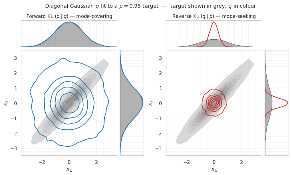
6. Forward vs reverse KL — mode-covering vs mode-seeking¶

What it is. Equation ((11)) is asymmetric — swapping $p$ and $q$ gives a different answer. Which direction you minimise determines which mismatches between $p$ and $q$ get punished most:

Forward / inclusive / zero-avoiding: $\mathrm{KL}(p\Vert q)$ blows up wherever $p > 0$ but $q\to 0$ . So the optimal $q$ ends up mode-covering — it spreads to cover all of $p$ ’s support, even at the cost of putting mass where $p$ is small.
Reverse / exclusive / zero-forcing: $\mathrm{KL}(q\Vert p)$ blows up wherever $q > 0$ but $p\to 0$ . So the optimal $q$ ends up mode-seeking — it concentrates on the densest region(s) and ignores the rest.

Continuous-form recipes for the optimal diagonal-Gaussian fit. Restrict $q$ to mean-field $\mathcal{N}(\mathbf{m}, \mathrm{diag}(\sigma_i^2))$ with $p = \mathcal{N}(\boldsymbol{\mu}_p, \boldsymbol{\Sigma}_p)$ . The closed-form optima are

\mathrm{argmin}_q \,\mathrm{KL}(p\,\Vert\,q): \quad \mathbf{m}^* = \boldsymbol{\mu}_p, \quad \sigma_i^{*\,2} = (\boldsymbol{\Sigma}_p)_{ii},

((12))

\mathrm{argmin}_q \,\mathrm{KL}(q\,\Vert\,p): \quad \mathbf{m}^* = \boldsymbol{\mu}_p, \quad \sigma_i^{*\,2} = 1/[\boldsymbol{\Sigma}_p^{-1}]_{ii}.

((13))

Equation ((12)) matches marginal variances; equation ((13)) matches conditional precisions. The two recipes give qualitatively different σ’s whenever $\boldsymbol{\Sigma}_p$ has off-diagonal mass, and are identical only when the target is already diagonal.

Numerical recipe. Equations ((12)) and ((13)) are one-liners — diagonal of $\boldsymbol{\Sigma}_p$ for the forward fit, diagonal of $\boldsymbol{\Sigma}_p^{-1}$ for the reverse fit. The plot below uses these analytic fits directly; no optimisation loop needed.

Interpretation & where it shows up.

Reverse KL is the VI default. Standard ELBO-based VI minimises $\mathrm{KL}(q\Vert p_{\text{post}})$ because $-\mathrm{KL}(q\Vert p) \le \log p(\mathbf{y})$ gives a tractable lower bound on the marginal likelihood. The price is the mode-seeking pathology.
Variance under-estimation. ((13)) shows $\sigma_i^{*\,2}$ is the conditional variance, which is always less than the marginal variance of ((12)) when $\boldsymbol{\Sigma}_p$ has off-diagonal mass. This is the formal reason “vanilla VI underestimates posterior variance”.
Expectation propagation, α-divergences. EP locally minimises forward KL, getting mode-covering behaviour at the cost of a fixed-point iteration. α-divergences interpolate between the two directions, with α = 0 ↔ reverse KL and α = 1 ↔ forward KL.

# Target: strongly correlated 2D Gaussian.
mu_target = jnp.zeros(2)
Sigma_target = jnp.array([[1.0, 0.95],
                          [0.95, 1.0]])
target = MultivariateNormal(mu_target, psd_op(Sigma_target))

# Best diagonal Gaussian q = N(m, diag(s²)) under each KL direction.
# Forward KL(p || q):  m* = mu_p,   s_i*² = Σ_p,ii   (matches marginal moments)
# Reverse KL(q || p):  m* = mu_p,   s_i*² = 1/[Σ_p^{-1}]_{ii}  (matches conditional precisions)
m_fwd = mu_target
s_fwd = jnp.sqrt(jnp.diag(Sigma_target))                   # marginal stds
m_rev = mu_target
s_rev = jnp.sqrt(1.0 / jnp.diag(jnp.linalg.inv(Sigma_target)))  # conditional stds

print(f"forward KL fit : std = {np.asarray(s_fwd)}")
print(f"reverse KL fit : std = {np.asarray(s_rev)}")

forward KL fit : std = [1. 1.]
reverse KL fit : std = [0.3122499 0.3122499]

# Joint + marginal view via seaborn KDEs — the differences live in the marginals.
import matplotlib.gridspec as gs
import seaborn as sns

# Snapshot rcParams BEFORE seaborn's set_theme so we can restore them no matter
# what happens in the plotting block below — see the matching restore at the end
# of this cell. Earlier this used a try/finally pattern via a snapshot+restore;
# now we keep the snapshot on a copy of the *current* rcParams (post our cell-1
# setup) so any plotting-side exception cannot leak the seaborn whitegrid theme
# to later cells (which would silently kill major+minor grids in cells 22/24).
_RC_SNAPSHOT = plt.rcParams.copy()
sns.set_theme(style="whitegrid")
plt.rcParams.update({
    "axes.grid.which": "both",
    "xtick.minor.visible": True,
    "ytick.minor.visible": True,
    "grid.alpha": 0.3,
})
try:

    N_VIS = 8000
    key_p, key_f, key_r = jax.random.split(jax.random.PRNGKey(42), 3)
    samples_p   = np.asarray(target.sample(key_p, (N_VIS,)))
    samples_fwd = np.asarray(jax.random.normal(key_f, (N_VIS, 2))) * np.asarray(s_fwd) + np.asarray(m_fwd)
    samples_rev = np.asarray(jax.random.normal(key_r, (N_VIS, 2))) * np.asarray(s_rev) + np.asarray(m_rev)

    LIM = (-3.5, 3.5)

    def joint_panel(fig, outer, samples_target, samples_q, color_q, title):
        """Build a 2x2 gridspec inside ``outer``: top + right marginals around a central joint."""
        inner = gs.GridSpecFromSubplotSpec(
            2, 2, subplot_spec=outer,
            width_ratios=[4, 1], height_ratios=[1, 4],
            wspace=0.05, hspace=0.05,
        )
        ax_top   = fig.add_subplot(inner[0, 0])
        ax_main  = fig.add_subplot(inner[1, 0])
        ax_right = fig.add_subplot(inner[1, 1])

        # central joint: target as filled grey KDE, q overlaid as coloured outlines
        sns.kdeplot(x=samples_target[:, 0], y=samples_target[:, 1],
                    ax=ax_main, fill=True, levels=8,
                    color="0.4", alpha=0.6, thresh=0.02)
        sns.kdeplot(x=samples_q[:, 0], y=samples_q[:, 1],
                    ax=ax_main, fill=False, levels=6,
                    color=color_q, linewidths=1.6, thresh=0.02)
        ax_main.set_xlim(*LIM); ax_main.set_ylim(*LIM)
        ax_main.set_xlabel(r"$x_1$"); ax_main.set_ylabel(r"$x_2$")
        ax_main.minorticks_on()
        ax_main.grid(True, which="major", alpha=0.35, lw=0.6)
        ax_main.grid(True, which="minor", alpha=0.15, lw=0.4)

        # top marginal — x_1
        sns.kdeplot(x=samples_target[:, 0], ax=ax_top, color="0.4", fill=True, alpha=0.5)
        sns.kdeplot(x=samples_q[:, 0],      ax=ax_top, color=color_q, lw=1.6)
        ax_top.set_xlim(*LIM); ax_top.set_yticks([])
        ax_top.set_xticklabels([]); ax_top.set_xlabel(""); ax_top.set_ylabel("")
        ax_top.set_title(title, fontsize=11)

        # right marginal — x_2
        sns.kdeplot(y=samples_target[:, 1], ax=ax_right, color="0.4", fill=True, alpha=0.5)
        sns.kdeplot(y=samples_q[:, 1],      ax=ax_right, color=color_q, lw=1.6)
        ax_right.set_ylim(*LIM); ax_right.set_xticks([])
        ax_right.set_yticklabels([]); ax_right.set_xlabel(""); ax_right.set_ylabel("")


    fig = plt.figure(figsize=(11, 5.6))
    outer = gs.GridSpec(1, 2, figure=fig, wspace=0.18, top=0.88)

    joint_panel(fig, outer[0, 0], samples_p, samples_fwd,
                color_q="#1f77b4",
                title=r"Forward KL $(p\,\Vert\,q)$ — mode-covering")
    joint_panel(fig, outer[0, 1], samples_p, samples_rev,
                color_q="#d62728",
                title=r"Reverse KL $(q\,\Vert\,p)$ — mode-seeking")

    fig.suptitle(r"Diagonal Gaussian $q$ fit to a $\rho = 0.95$ target  —  "
                 r"target shown in grey, $q$ in colour",
                 fontsize=12, y=0.98)
    plt.show()
finally:
    # Restore pre-seaborn rcParams unconditionally — even if the plotting
    # above raises. This guarantees cells 22 / 24 keep their major+minor grids.
    plt.rcParams.update(_RC_SNAPSHOT)

7. The `kl_standard_normal` shortcut¶

What it is. A specialisation of equation ((11)) when $q = \mathcal{N}(\mathbf{0}, \mathbf{I})$ . The cross-terms vanish: $\boldsymbol{\Sigma}_q^{-1} = \mathbf{I}$ , $\boldsymbol{\mu}_q = \mathbf{0}$ , $\log\lvert\boldsymbol{\Sigma}_q\rvert = 0$ .

Continuous form.

\mathrm{KL}\!\bigl(\mathcal{N}(\mathbf{m}, \boldsymbol{\Sigma}) \,\Vert\, \mathcal{N}(\mathbf{0}, \mathbf{I})\bigr) = \tfrac{1}{2}\bigl[\mathrm{tr}(\boldsymbol{\Sigma}) + \mathbf{m}^\top\mathbf{m} - d - \log\lvert\boldsymbol{\Sigma}\rvert\bigr].

((14))

Numerical recipe. For diagonal $\boldsymbol{\Sigma} = \mathrm{diag}(\sigma_1^2, \dots, \sigma_d^2)$ equation ((14)) further specialises to

\mathrm{KL} = \tfrac{1}{2}\sum_i \bigl(\sigma_i^2 + m_i^2 - 1 - \log\sigma_i^2\bigr),

((15))

which is the per-coordinate formula you’ll see hard-coded in 90% of ELBO implementations.

Interpretation & where it shows up.

VAE prior regulariser. The KL term in the standard VAE loss is exactly equation ((15)) summed across latent dimensions and batched across data points.
Whitening. SVGP and Bayesian NN methods often change variables to make the prior $\mathcal{N}(\mathbf{0}, \mathbf{I})$ — every KL becomes equation ((14)) and stays cheap.
Easy gradients. The diagonal form ((15)) is per-coordinate and trivially differentiable, which is why mean-field variational families default to this parameterisation. Compare to the full equation ((11)), where the Cholesky of $\boldsymbol{\Sigma}_q$ shows up in every gradient.

m = jnp.array([0.5, -0.25])
S_diag = jnp.array([[0.6, 0.0],
                    [0.0, 1.4]])
S = psd_op(S_diag)
I_d = psd_op(jnp.eye(2))

# (a) gaussx shortcut.
KL_short = float(kl_standard_normal(m, S))

# (b) general routine via dist_kl_divergence.
KL_full = float(dist_kl_divergence(m, S, jnp.zeros(2), I_d))

# (c) hand-rolled diagonal formula via einx.
sigma2 = jnp.diag(S_diag)
KL_diag = 0.5 * float(einx.sum("i ->", sigma2 + m * m - 1.0 - jnp.log(sigma2)))

print(f"kl_standard_normal       : {KL_short:.6f}")
print(f"dist_kl_divergence vs N(0,I): {KL_full:.6f}")
print(f"hand-rolled diagonal     : {KL_diag:.6f}")

kl_standard_normal       : 0.243427
dist_kl_divergence vs N(0,I): 0.243427
hand-rolled diagonal     : 0.243427

8. Expected log-likelihood under a Gaussian¶

What it is. When the latent variable $\mathbf{f}$ is itself uncertain (described by a Gaussian variational posterior $q(\mathbf{f}) = \mathcal{N}(\boldsymbol{\mu}_q, \boldsymbol{\Sigma}_q)$ ), and the observation model is Gaussian $p(\mathbf{y}\mid\mathbf{f}) = \mathcal{N}(\mathbf{f}, \mathbf{R})$ , the data-fit term of the ELBO has a closed form that decomposes into “log-density at the mean” plus a “trace correction” for posterior uncertainty.

Continuous form.

\mathbb{E}_q[\log p(\mathbf{y}\mid\mathbf{f})] = -\tfrac{m}{2}\log 2\pi - \tfrac{1}{2}\log\lvert\mathbf{R}\rvert - \tfrac{1}{2}(\mathbf{y}-\boldsymbol{\mu}_q)^\top\mathbf{R}^{-1}(\mathbf{y}-\boldsymbol{\mu}_q) - \tfrac{1}{2}\mathrm{tr}(\mathbf{R}^{-1}\boldsymbol{\Sigma}_q).

((16))

The first three terms are just the log-density of a Gaussian (cf. 0.1 §1) evaluated at the posterior mean. The fourth — the trace correction $\tfrac{1}{2}\mathrm{tr}(\mathbf{R}^{-1}\boldsymbol{\Sigma}_q)$ — is new.

Numerical recipe. All four terms reuse the same Cholesky of $\mathbf{R}$ :

\mathbb{E}_q[\log p(\mathbf{y}\mid\mathbf{f})] = \log\mathcal{N}(\mathbf{y}; \boldsymbol{\mu}_q, \mathbf{R}) - \tfrac{1}{2}\mathrm{tr}(\mathbf{R}^{-1}\boldsymbol{\Sigma}_q).

((17))

The trace can be written $\mathrm{tr}(\mathbf{L}_R^{-1}\boldsymbol{\Sigma}_q\mathbf{L}_R^{-\top})$ with $\mathbf{R} = \mathbf{L}_R\mathbf{L}_R^\top$ , sharing factors with ((2)) and ((6)).

Interpretation & where it shows up.

Trace correction = “uncertainty tax”. It vanishes as $\boldsymbol{\Sigma}_q\to\mathbf{0}$ (deterministic limit) and grows as $\boldsymbol{\Sigma}_q$ inflates. So an over-confident $q$ — small $\boldsymbol{\Sigma}_q$ — has a small ELL penalty but pays through the KL term ((11)); an over-spread $q$ is the opposite. Balancing the two is what variational fitting does.
SVGP / VGP / Bayesian NN ELBOs. Every Gaussian-likelihood variational ELBO has equation ((16)) (or its sum across data points) as its data-fit term.
Conjugate identity. When $q$ equals the true Gaussian-conjugate posterior, equation ((16)) plus the prior KL ((11)) collapses to $\log p(\mathbf{y})$ — the marginal likelihood of the data. We see this concretely in §10.

gaussx.gaussian_expected_log_lik(y, q_mu, q_cov, noise) evaluates equation ((16)) directly.

# Mock data: 3-dim observation y, latent f ~ N(q_mu, q_cov), noise R.
y = jnp.array([1.0, 0.5, -0.3])
q_mu_f = jnp.array([0.9, 0.6, -0.2])
q_cov_f = psd_op(0.05 * jnp.eye(3) + 0.02)
R = psd_op(0.1 * jnp.eye(3))

ELL_gx = float(gaussian_expected_log_lik(y, q_mu_f, q_cov_f, R))

# Closed-form check term-by-term, written with einx.
m_obs = y.shape[0]
delta_y = y - q_mu_f
R_dense = R.as_matrix()
quad_term = float(quadratic_form(R, delta_y))
trace_term = float(jnp.trace(jnp.linalg.solve(R_dense, q_cov_f.as_matrix())))
_, logdet_R = jnp.linalg.slogdet(R_dense)
ELL_manual = -0.5 * m_obs * jnp.log(2 * jnp.pi) - 0.5 * logdet_R \
             - 0.5 * quad_term - 0.5 * trace_term

# Monte-Carlo cross-check.
key = jax.random.PRNGKey(123)
q_dist = MultivariateNormal(q_mu_f, q_cov_f)
f_samples = q_dist.sample(key, (50_000,))
def loglik(f):
    return gaussian_log_prob(f, R, y)
ELL_mc = float(jnp.mean(jax.vmap(loglik)(f_samples)))

print(f"ELL (gaussx primitive)   : {ELL_gx:.6f}")
print(f"ELL (manual closed form) : {float(ELL_manual):.6f}")
print(f"ELL (MC, 50k samples)    : {ELL_mc:.6f}")

ELL (gaussx primitive)   : -0.502938
ELL (manual closed form) : -0.502938
ELL (MC, 50k samples)    : -0.500431

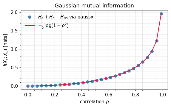
9. Mutual information between blocks¶

What it is. Mutual information $I(X_a; X_b) = H(X_a) + H(X_b) - H(X_a, X_b)$ measures the reduction in uncertainty about $X_a$ obtained by observing $X_b$ (and vice versa — it’s symmetric, despite KL not being). For Gaussians the entropies all simplify via equation ((5)), leaving a ratio of log-determinants.

Continuous form. Partition $\mathbf{x} = (\mathbf{x}_a, \mathbf{x}_b)$ as in 0.1 §4. Substituting equation ((5)) for each entropy term and cancelling the additive constants:

I(X_a; X_b) = \tfrac{1}{2}\log\!\frac{\lvert\boldsymbol{\Sigma}_{aa}\rvert\,\lvert\boldsymbol{\Sigma}_{bb}\rvert}{\lvert\boldsymbol{\Sigma}\rvert}.

((18))

Numerical recipe. Three log-determinants, no quadratic forms — equation ((18)) is computed entirely from Cholesky factors of $\boldsymbol{\Sigma}_{aa}$ , $\boldsymbol{\Sigma}_{bb}$ , and the joint $\boldsymbol{\Sigma}$ . For the 2D case with correlation ρ it collapses to

I(X_a; X_b) = -\tfrac{1}{2}\log(1 - \rho^2),

((19))

a recovery of the classical information-theoretic measure of correlation strength.

Interpretation & where it shows up.

Conditional independence. $I(X_a; X_b) = 0$ iff $\boldsymbol{\Sigma}_{ab} = \mathbf{0}$ , in which case the joint factorises as the product of marginals. Equation ((18)) is therefore a quantitative diagnostic for how strongly two blocks interact — exactly the question Gaussian graphical models try to answer.
Sensor placement / experimental design. Choose observations $\mathbf{x}_b$ that maximise $I$ with the quantity of interest $\mathbf{x}_a$ — equivalently, that shrink the determinant of the conditional covariance via the Schur identity from 0.1 §5.
Bayesian active learning. Predictive entropy search and BALD use equation ((18)) (often with a non-Gaussian likelihood, but Gaussian-approximated) to score candidate queries.
Information bottleneck. The IB objective is a difference of MI terms; for Gaussian-process variants both pieces have closed forms via ((18)).

rhos = jnp.linspace(0.0, 0.99, 30)

def mi_2d(rho: float) -> float:
    Sigma = jnp.array([[1.0, rho], [rho, 1.0]])
    Sigma_aa = psd_op(Sigma[:1, :1])
    Sigma_bb = psd_op(Sigma[1:, 1:])
    Sigma_full = psd_op(Sigma)
    H_aa = float(gaussian_entropy(Sigma_aa))
    H_bb = float(gaussian_entropy(Sigma_bb))
    H_full = float(gaussian_entropy(Sigma_full))
    return H_aa + H_bb - H_full

mi_vals = jnp.array([mi_2d(float(r)) for r in rhos])
mi_closed = -0.5 * jnp.log(1.0 - rhos ** 2)

fig, ax = plt.subplots(figsize=(5.4, 3.4))
ax.plot(np.asarray(rhos), np.asarray(mi_vals), "o", label=r"$H_a + H_b - H_{ab}$ via gaussx", color="steelblue")
ax.plot(np.asarray(rhos), np.asarray(mi_closed), "-", label=r"$-\frac{1}{2}\log(1-\rho^2)$", color="crimson")
ax.set_xlabel(r"correlation $\rho$"); ax.set_ylabel(r"$I(X_a; X_b)$ [nats]")
ax.set_title("Gaussian mutual information")
ax.legend(frameon=False)
plt.tight_layout(); plt.show()

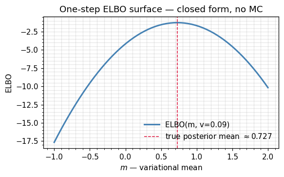
10. Putting it together: a one-step ELBO¶

What it is. The Evidence Lower BOund (ELBO) is the workhorse of variational inference. It decomposes as data-fit minus prior penalty: the expected log-likelihood ((16)) of the data under $q$ , minus the KL ((11)) between $q$ and the prior.

Continuous form.

\mathrm{ELBO}(q) = \underbrace{\mathbb{E}_q[\log p(\mathbf{y}\mid\mathbf{f})]}_{\text{data fit}} \;-\; \underbrace{\mathrm{KL}\!\bigl(q(\mathbf{f}) \,\Vert\, p(\mathbf{f})\bigr)}_{\text{prior penalty}}.

((20))

Numerical recipe. Plug equation ((16)) and equation ((11)) into ((20)). Both pieces share Cholesky factors with everything in this notebook. For the toy below we sweep $q$ ’s mean over a grid; in real use you’d differentiate the ELBO and run gradient ascent — every term in the gradient is also closed-form.

Interpretation.

Variational identity. $\log p(\mathbf{y}) - \mathrm{ELBO}(q) = \mathrm{KL}(q\Vert p_{\text{post}}) \ge 0$ , with equality iff $q$ equals the true posterior. Maximising the ELBO over $q$ minimises the variational gap.
Conjugate sanity check. For Gaussian-Gaussian conjugate models, the optimum $q$ is the true posterior, and the ELBO equals $\log p(\mathbf{y})$ exactly. The toy below illustrates this: the ELBO peak lands on the conjugate posterior mean.
Scales linearly. Add data points → sum more gaussian_expected_log_lik terms; add latent dimensions → bigger Cholesky. No new closed forms ever needed.

y_obs = jnp.array([0.8])
prior_mu = jnp.zeros(1)
prior_cov = psd_op(jnp.eye(1))
noise = psd_op(0.1 * jnp.eye(1))

def elbo(q_m: float, q_v: float) -> float:
    q_mu_arr = jnp.array([q_m])
    q_cov = psd_op(q_v * jnp.eye(1))
    ell = gaussian_expected_log_lik(y_obs, q_mu_arr, q_cov, noise)
    kl = dist_kl_divergence(q_mu_arr, q_cov, prior_mu, prior_cov)
    return float(ell - kl)

q_means = jnp.linspace(-1.0, 2.0, 60)
q_var = 0.09
elbos = jnp.array([elbo(float(m), q_var) for m in q_means])

# True posterior mean for a Gaussian-Gaussian conjugate pair (closed form).
post_var = 1.0 / (1.0 / 1.0 + 1.0 / 0.1)
post_mean = post_var * (0.0 / 1.0 + 0.8 / 0.1)
print(f"true posterior     : N({post_mean:.4f}, {post_var:.4f})")
print(f"argmax ELBO over m : {float(q_means[jnp.argmax(elbos)]):.4f}")

fig, ax = plt.subplots(figsize=(5.4, 3.4))
ax.plot(np.asarray(q_means), np.asarray(elbos), color="steelblue", lw=2, label="ELBO(m, v=0.09)")
ax.axvline(post_mean, color="crimson", ls="--", lw=1, label=fr"true posterior mean $\approx {post_mean:.3f}$")
ax.set_xlabel(r"$m$ — variational mean"); ax.set_ylabel("ELBO")
ax.set_title("One-step ELBO surface — closed form, no MC")
ax.legend(frameon=False)
plt.tight_layout(); plt.show()

true posterior     : N(0.7273, 0.0909)

argmax ELBO over m : 0.7288

11. Recap & where to go next¶

Quantity	Continuous form (equation)	Numerical (equation)	gaussx entry point
Quadratic form	((1))	((2))	`quadratic_form`
Score	((3))	((4))	`solve` (or `jax.grad` of `gaussian_log_prob`)
Entropy	((5))	((6))	`gaussian_entropy`
Cross-entropy	((8))	via identity ((9))	$H(p) + \mathrm{KL}(p\Vert q)$
KL divergence	((11))	reuses Cholesky factors	`dist_kl_divergence`
KL vs $\mathcal{N}(0,I)$	((14))	diagonal: ((15))	`kl_standard_normal`
Expected log-likelihood	((16))	((17))	`gaussian_expected_log_lik`
Mutual information	((18))	2D special case ((19))	sum of `gaussian_entropy` calls
ELBO	((20))	ELL − KL	combine the two above

Next up.

0.4 — Mean-cov ↔ natural parameter conversions: the third equivalent representation, plus log_partition, fisher_info, and the Bregman view of KL.
0.7 — Conditional distributions & Schur complement: full treatment of Gaussian conditioning.
Part 5 — Variational approximations: where these closed forms are summed over data to give the SVGP / VGP / variational Bayes machinery.

Quadratic forms, entropy, KL — closed-form Gaussian quantities

1. The quadratic form δ⊤Σ−1δ\delta^\top \boldsymbol{\Sigma}^{-1}\deltaδ⊤Σ−1δ¶

2. The score ∇xlog⁡p(x)\nabla_{\mathbf{x}}\log p(\mathbf{x})∇x​logp(x)¶

3. Entropy¶

4. Cross-entropy and the H / KL / cross-entropy identity¶

5. KL between two Gaussians¶

6. Forward vs reverse KL — mode-covering vs mode-seeking¶

7. The kl_standard_normal shortcut¶

8. Expected log-likelihood under a Gaussian¶

9. Mutual information between blocks¶

10. Putting it together: a one-step ELBO¶

11. Recap & where to go next¶

1. The quadratic form $\delta^\top \boldsymbol{\Sigma}^{-1}\delta$ ¶

2. The score $\nabla_{\mathbf{x}}\log p(\mathbf{x})$ ¶

7. The `kl_standard_normal` shortcut¶