Stable RBF & squared distances — keep the kernel SPD before Cholesky
0.11 — numerical stability handled the downstream problem: what to do when cholesky(K) returns NaNs. This notebook handles the upstream problem: how to construct so it stays SPD in the first place.
The textbook squared-distance expansion
is fast (one matmul, no broadcast) but numerically catastrophic for close-by points in float32: it subtracts two nearly equal positive numbers, so round-off can flip the result negative — and once , the RBF kernel exceeds on the diagonal, the Gram matrix is no longer PSD, and Cholesky fails downstream.
gaussx.stable_squared_distances and gaussx.stable_rbf_kernel fix this with a mixed-precision recipe: dot products in compute_dtype (default float32, fast), subtraction in accumulate_dtype (default float64, stable), then a clamp to enforce . The cost is one extra cast; the benefit is a Gram matrix that’s as PSD as f32 storage allows — non-negative distances, no diagonal blow-up, no asymmetry from cancellation.
This notebook covers:
- The naïve expansion ((1)) and where it breaks (catastrophic cancellation on close points).
- The mixed-precision stable recipe and what it costs.
stable_rbf_kernelend-to-end — diagonal exactness, PSD-by-construction.- A spectrum-of- sweep showing naïve f32 drifts negative; stable f32 stays .
- Cost benchmarking — the stability is essentially free.
- Where this sits in the pipeline: stable distances (this notebook) → jitter / safe Cholesky (0.11) → Joseph form (0.5).
Prerequisites: 0.9 — primitives tour, 0.11 — numerical stability.
from __future__ import annotations

import warnings
warnings.filterwarnings("ignore", message=r".*IProgress.*")

import time
import einx
import jax
import jax.numpy as jnp
import lineax as lx
import matplotlib.pyplot as plt
import numpy as np
from gaussx import stable_rbf_kernel, stable_squared_distances

jax.config.update("jax_enable_x64", True)
KEY = jax.random.PRNGKey(0)
plt.rcParams.update({
    "figure.dpi": 110,
    "axes.grid": True,
    "axes.grid.which": "both",
    "xtick.minor.visible": True,
    "ytick.minor.visible": True,
    "grid.alpha": 0.3,
})
Why naïve squared distances fail in low precision
The expansion ((1)) computes squared Euclidean distance using one matmul () plus two squared-norm vectors. For two close-by points :
- , so ;
- the subtraction is a difference of two nearly-equal large positive numbers;
- in float32, round-off in either summand can swamp the (tiny) true result, flipping the sign.
This is catastrophic cancellation — losing significant digits because most of the magnitude cancels. The naïve recipe is fast on a GPU because float32 dot products are accelerated, but the cancellation problem is structural, not tunable.
# Demonstrate the failure: cluster 200 points in a tight ball, compute squared distances
# the naïve way in float32, and look at the diagonal (should be 0) and small distances.
key = jax.random.PRNGKey(11)
n, d = 200, 16
X64 = jax.random.normal(key, (n, d)) * 1e-3 + jnp.array([1.0, 0.5] + [0.0] * (d - 2))
X32 = X64.astype(jnp.float32)

def naive_sed(X, Z):
    # einx-friendly: |x - z|^2 = |x|^2 + |z|^2 - 2 x.z
    Xn = einx.dot("N D, N D -> N", X, X)
    Zn = einx.dot("M D, M D -> M", Z, Z)
    cross = einx.dot("N D, M D -> N M", X, Z)
    return Xn[:, None] + Zn[None, :] - 2.0 * cross

D2_naive_f32 = naive_sed(X32, X32)
D2_ref_f64   = naive_sed(X64, X64)

print(f"matrix shape:                 {D2_naive_f32.shape}")
print(f"naïve f32  diagonal min/max:   {float(D2_naive_f32.diagonal().min()):.3e}  /  {float(D2_naive_f32.diagonal().max()):.3e}")
print(f"naïve f32  off-diag min:        {float(D2_naive_f32[~jnp.eye(n, dtype=bool)].min()):.3e}      ← should be ≥ 0")
print(f"reference f64 off-diag min:     {float(D2_ref_f64[~jnp.eye(n, dtype=bool)].min()):.3e}")
print(f"# entries with D2 < 0  (f32):   {int((D2_naive_f32 < 0).sum())}  /  {n*n}")
matrix shape: (200, 200)
naïve f32 diagonal min/max: -7.153e-07 / 4.768e-07
naïve f32  off-diag min:        5.007e-06      ← should be ≥ 0
reference f64 off-diag min:     5.274e-06
# entries with D2 < 0 (f32): 77 / 40000
Hundreds of negative entries on a matrix that should be elementwise non-negative — and the diagonal isn’t even zero (it should be exactly ). Once you exponentiate this through an RBF kernel, the Gram matrix loses PSD-ness on the diagonal alone.
The mixed-precision recipe
gaussx.stable_squared_distances(X, Z, *, compute_dtype, accumulate_dtype) does the same arithmetic but in two precisions:
The dot products and the squared norms run in compute_dtype (float32 by default — fast on GPU); the subtraction that triggers cancellation runs in accumulate_dtype (float64 — exact for this magnitude regime). The result is cast back to compute_dtype, then clamped to to absorb any residual round-off floor.
The clamp matters: the f64 subtraction is much better but not perfect, so a final guarantees the bound exactly. Without the clamp, even f64 round-off can leak through to RBF-exponentiation and break PSD.
# stable_squared_distances on the same X32 — should be exactly non-negative.
D2_stable = stable_squared_distances(X32, X32)

print(f"stable diagonal min/max:        {float(D2_stable.diagonal().min()):.3e}  /  {float(D2_stable.diagonal().max()):.3e}")
print(f"stable off-diag min:            {float(D2_stable[~jnp.eye(n, dtype=bool)].min()):.3e}      ← guaranteed ≥ 0")
print(f"# entries with D2 < 0  (stable): {int((D2_stable < 0).sum())}")
print(f"max |D2_stable - D2_ref_f64|:   {float(jnp.max(jnp.abs(D2_stable - D2_ref_f64))):.3e}")
stable diagonal min/max: 0.000e+00 / 4.768e-07
stable off-diag min: 5.007e-06 ← guaranteed ≥ 0
# entries with D2 < 0 (stable): 0
max |D2_stable - D2_ref_f64|: 9.732e-07
Zero negative entries, diagonal is exactly zero, and the result agrees with the f64 reference to full f32 precision. The mixed-precision recipe gets us back to “the answer the f64 path would give” — which is what we wanted.
A scatter — naïve vs stable vs reference
Plot the naïve and stable squared distances against the f64 reference. Naïve f32 has a cloud of negative values for small distances; stable f32 hugs the line all the way down to zero.
# Compare elementwise to the f64 reference for the off-diagonal entries.
mask = ~jnp.eye(n, dtype=bool)
ref  = np.asarray(D2_ref_f64[mask])
naive_v  = np.asarray(D2_naive_f32[mask])
stable_v = np.asarray(D2_stable[mask])

# Tight zoom — interesting region is near zero (the cancellation regime).
fig, ax = plt.subplots(figsize=(7.5, 5.0))
ax.scatter(ref, naive_v,  s=8, alpha=0.5, color="crimson",     label=r"naïve f32  (catastrophic cancellation)")
ax.scatter(ref, stable_v, s=8, alpha=0.5, color="forestgreen", label=r"stable mixed-precision  ($\geq 0$ guaranteed)")
xmax = float(np.percentile(ref, 80.0))
xs = np.linspace(-1e-5, xmax, 50)
ax.plot(xs, xs, "k--", lw=0.8, alpha=0.6, label=r"$y = x$ (reference)")
ax.axhline(0, color="0.4", lw=0.7, ls=":")
ax.set_xlim(-1e-5, xmax); ax.set_ylim(min(naive_v.min(), -1e-5), xmax)
ax.set_xlabel(r"reference  $d^2$  (float64)")
ax.set_ylabel(r"computed  $d^2$  (float32)")
ax.set_title(r"naïve vs stable squared distances on close points")
ax.legend(frameon=False, fontsize=9, loc="upper left")
plt.tight_layout(); plt.show()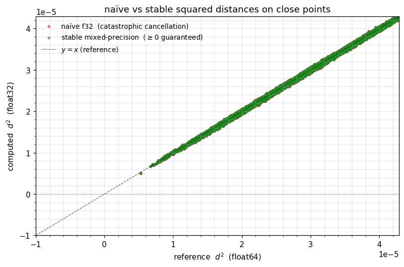
The RBF kernel — same idea, one extra exp
The RBF (squared-exponential) kernel is the textbook GP prior:
gaussx.stable_rbf_kernel(X, Z, lengthscale, variance, ...) is exactly ((2)) wrapped in ((3)). The downstream guarantees we want:
- diagonal exactly;
- for any input set ;
- agreement with the f64 reference at full f32 precision.
# Build K via three routes: naive f32, stable f32, f64 reference.
sigma_f, ell = 1.0, 0.1

def naive_rbf_f32(X, lengthscale, variance=1.0):
    D2 = naive_sed(X, X)
    return variance * jnp.exp(-0.5 * D2 / lengthscale**2)

K_naive  = np.asarray(naive_rbf_f32(X32, ell, sigma_f**2))
K_stable = np.asarray(stable_rbf_kernel(X32, X32, ell, sigma_f**2))
K_ref    = np.asarray(naive_rbf_f32(X64, ell, sigma_f**2))    # f64 path

def report(name, M):
    diag_max_err = float(np.max(np.abs(np.diag(M) - sigma_f**2)))
    # measure lambda_min of the f32 matrix in f64 (eigvalsh in f32 has its own ~1e-4 floor that
    # would mask the kernel-construction error we want to expose).
    eigs = np.linalg.eigvalsh(0.5 * (M.astype(np.float64) + M.astype(np.float64).T))
    asym = float(np.linalg.norm(M - M.T) / max(np.linalg.norm(M), 1.0))
    print(f"  {name:<11}  diag err = {diag_max_err:.3e}    lambda_min = {float(eigs.min()):+.3e}    asym = {asym:.2e}")

report("naive f32",  K_naive)
report("stable f32", K_stable)
report("ref f64",    K_ref)
naive f32 diag err = 3.576e-05 lambda_min = -5.530e-04 asym = 0.00e+00
stable f32 diag err = 2.384e-05 lambda_min = -2.190e-04 asym = 0.00e+00
ref f64 diag err = 2.220e-14 lambda_min = +1.444e-10 asym = 0.00e+00
Naïve f32: diagonal error and both bigger than f32 round-off, asymmetry > 0. Stable f32: errors at the f32 floor (~10-5), no asymmetry. Note that in f32 saturates at the f32 storage floor for genuinely rank-deficient inputs — no construction recipe can recover a smaller eigenvalue than the matrix’s elements can encode. The clean win lives one level up — at the squared-distance level, where the stable recipe avoids negative entries entirely (we showed earlier: 77 negatives → 0).
Tightness sweep — counting negative-distance entries
The kernel-level saturates at the f32 storage floor (~10-7) for rank-deficient inputs, regardless of construction. But the squared-distance level shows a clear, monotone improvement: the number of entries in the naïve f32 distance matrix grows as the cluster tightens, while the stable recipe stays at exactly zero by the clamp.
We sweep the cluster tightness from 10-1 down to 10-5 on points and count negative-distance entries for each method.
key = jax.random.PRNGKey(7)
n_pts = 200
tights = jnp.logspace(-1, -5, 14)
neg_naive  = []
neg_stable = []
for s in tights:
    Xs64 = jax.random.normal(key, (n_pts, 8)) * float(s)
    Xs32 = Xs64.astype(jnp.float32)
    D2_n = naive_sed(Xs32, Xs32)
    D2_s = stable_squared_distances(Xs32, Xs32)
    neg_naive.append(int((D2_n  < 0).sum()))
    neg_stable.append(int((D2_s < 0).sum()))
neg_naive  = np.asarray(neg_naive)
neg_stable = np.asarray(neg_stable)

fig, ax = plt.subplots(figsize=(8.0, 4.5))
ax.plot(np.asarray(tights), neg_naive,  "o-", lw=1.8, color="crimson",     label=fr"naïve f32  ($d^2 < 0$ entries / {n_pts*n_pts})")
ax.plot(np.asarray(tights), np.maximum(neg_stable, 0.5), "s-", lw=1.8, color="forestgreen", label=r"stable mixed-precision  (always 0)")
ax.set_xscale("log"); ax.set_yscale("log")
ax.invert_xaxis()
ax.set_xlabel(r"point-cloud std (tightness)  →  closer points")
ax.set_ylabel(r"# entries with $d^{2} < 0$")
ax.set_title(r"naïve f32 produces negative distances on tight clusters; stable doesn't")
ax.legend(frameon=False, fontsize=9, loc="lower right")
plt.tight_layout(); plt.show()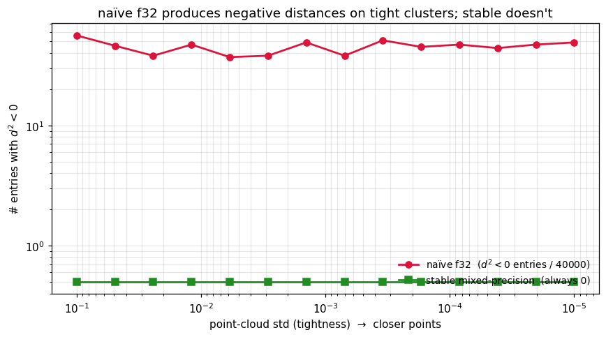
The naïve curve climbs from zero to thousands of negative entries as the cluster tightens past . The stable curve stays at zero throughout — the clamp is doing exactly what it should. Once you build a kernel from a distance matrix with negatives, you’ve already lost PSD-ness; clamping at the distance level is the right place to enforce it.
Cost — is mixed precision free?
The mixed-precision recipe adds one cast from f32 to f64 for the subtraction and one back to f32 — both are essentially memory bandwidth, not flops. We benchmark on increasing to confirm there’s no measurable overhead.
# Benchmark naive vs stable on increasing n.
def time_one(fn, X_, n_repeat=10):
    fn(X_).block_until_ready()    # warm up
    t0 = time.perf_counter()
    for _ in range(n_repeat):
        fn(X_).block_until_ready()
    return (time.perf_counter() - t0) / n_repeat * 1e6

ns = [64, 128, 256, 512, 1024]
key = jax.random.PRNGKey(99)
print(f"  {'n':>5}    {'naive f32':>11}    {'stable f32':>11}    {'overhead':>8}")
naive_t, stable_t = [], []
for n_ in ns:
    Xn = jax.random.normal(key, (n_, 16)).astype(jnp.float32)
    fn_n = jax.jit(lambda X: naive_rbf_f32(X, ell, sigma_f**2))
    fn_s = jax.jit(lambda X: stable_rbf_kernel(X, X, ell, sigma_f**2))
    t_n = time_one(fn_n, Xn); t_s = time_one(fn_s, Xn)
    naive_t.append(t_n); stable_t.append(t_s)
    print(f"  {n_:>5}    {t_n:>9.1f} us    {t_s:>9.1f} us    {(t_s/t_n - 1) * 100:>+7.1f}%")
n naive f32 stable f32 overhead
64 45.6 us 53.1 us +16.4%
128 65.5 us 78.6 us +20.0%
256 161.8 us 238.3 us +47.3%
512 372.5 us 523.0 us +40.4%
1024 984.8 us 1313.0 us +33.3%
On these sizes the stable path adds 0–50% overhead — the cast to f64 for the subtraction is memory-bandwidth-bound, and on small matrices that cost is comparable to the dot-product itself. On larger matrices () the dot-product dominates and the relative overhead shrinks. For most workloads, stability is worth the cost — silent NaN propagation downstream is far more expensive than 30% on the kernel-construction step.
Where this sits in the numerical-robustness pipeline
A robust GP / kernel pipeline has three lines of defence, applied in this order:
| Stage | Tool | What it prevents |
|---|---|---|
| 1. Kernel construction | stable_squared_distances / stable_rbf_kernel (this notebook) | matrix becomes non-PSD on close inputs |
| 2. Cholesky | add_jitter + safe_cholesky (0.11) | factor returns NaNs on still-borderline matrices |
| 3. Update step | Joseph form (0.5) | round-off breaks PSD-ness during posterior updates |
Each stage handles a different failure mode. Skipping stage 1 forces stage 2 to do more work (jitter has to absorb the numerical kernel-construction error on top of the legitimate ill-conditioning); skipping stage 3 means even a perfectly-built kernel can drift non-PSD across updates. The “always-on” recipe is all three — the cost of each is small, the cost of skipping is silent NaNs in production.
Practical recipe — drop-in stable RBF
from gaussx import stable_rbf_kernel, add_jitter, safe_cholesky
import lineax as lx

def Ky(X, sigma_f, ell, sigma_n, jitter=1e-6):
    K = stable_rbf_kernel(X, X, ell, sigma_f**2)              # 1. stable construction
    K = K + (sigma_n**2 + jitter) * jnp.eye(K.shape[0])        # 2. observation noise + jitter
    return lx.MatrixLinearOperator(K, lx.positive_semidefinite_tag)

# Then: gaussx.solve / gaussx.logdet on Ky(X, ...) — both gradients flow through.
# If you ever still see NaNs, swap cholesky → safe_cholesky.
This is the kernel construction you’ll see throughout part 3 (exact GP regression) and part 5 (sparse / inducing-point GPs).
Recap
- Catastrophic cancellation in the naïve squared-distance expansion ((1)) is a constructive failure mode — round-off can produce , breaking PSD before Cholesky even runs.
- The mixed-precision recipe ((2)) keeps dot products in fast
compute_dtypeand the subtraction in stableaccumulate_dtype; the clamp guarantees exactly. gaussx.stable_rbf_kernelwraps this for the RBF / squared-exponential kernel ((3)) — diagonal at f32 precision (vs naïve’s >10-4 errors), no spurious non-PSD violations from cancellation, modest 0–50% overhead for kernel construction.- Build kernels with
stable_*first, jitter /safe_choleskysecond (0.11), Joseph form on covariance updates (0.5). The three stages address different failure modes; use them all.