Differentiating through solve — implicit gradients for Gaussian inference

The fifth primitive — alongside cholesky / logdet / trace / diag from 0.9 — is solve. Unlike the other four, solve has no closed-form structural shortcut for its gradient: you can’t just sum logs of diagonal entries. Instead, lineax (the engine under gaussx.solve) registers a custom JVP / VJP with JAX that uses the implicit function theorem to give you the gradient with one additional solve, reusing the same factorisation.

This is the AD machinery that makes jax.grad “just work” through every Gaussian quantity in the curriculum: log-density ((6)), KL divergence, ELBO, GP marginal likelihood. You write the forward expression, JAX gives you the gradient — no need to derive Cholesky-derivative formulas by hand.

This notebook covers:

The implicit-function-theorem identity for $\partial x/\partial\theta$ when $A(\theta)x = b$ .
How lineax implements forward-mode (JVP) and reverse-mode (VJP) gradients of linear_solve, and why both reuse the same factor.
Jacobi’s formula for $\partial \log\lvert A\rvert / \partial\theta$ — the other half of the GP marginal-likelihood gradient.
End-to-end gradient descent through gaussx.solve to optimise a parameter.
The GP marginal-likelihood gradient as the natural application: jax.grad through one log-mlik evaluation gives all hyperparameter gradients.

Prerequisites: 0.3 — Gaussian quantities, 0.9 — primitives tour.

from __future__ import annotations

import warnings
warnings.filterwarnings("ignore", message=r".*IProgress.*")

import einx
import jax
import jax.numpy as jnp
import lineax as lx
import matplotlib.pyplot as plt
import numpy as np
import gaussx

jax.config.update("jax_enable_x64", True)
KEY = jax.random.PRNGKey(0)
plt.rcParams.update({
    "figure.dpi": 110,
    "axes.grid": True,
    "axes.grid.which": "both",
    "xtick.minor.visible": True,
    "ytick.minor.visible": True,
    "grid.alpha": 0.3,
})

def psd_op(M):
    return lx.MatrixLinearOperator(M, lx.positive_semidefinite_tag)

The implicit function theorem for linear systems¶

When parameters θ enter the matrix $A(\theta)$ in a linear system $A(\theta)\,x(\theta) = b$ , the solution $x(\theta)$ is defined implicitly. Differentiating both sides with respect to θ and rearranging gives

\frac{\partial x}{\partial \theta} \;=\; -\,A^{-1}\,\frac{\partial A}{\partial \theta}\,x.

((1))

The cost is one extra solve (with the same matrix $A$ ), not a full Jacobian computation. This is the implicit-function-theorem applied to the linear case, and it’s what lets jax.grad propagate gradients through gaussx.solve without ever materialising $\partial x / \partial \theta$ as a dense matrix.

Two flavours of AD use the same primitive:

\dot{x} \;=\; A^{-1}\bigl(\dot{b} - \dot{A}\,x\bigr) \qquad\text{(forward mode / JVP)}

((2))

\lambda \;=\; A^{-\top}\,\bar{x}, \qquad \bar{b} \;=\; \lambda, \qquad \bar{A}\colon \delta A \mapsto -\lambda^\top(\delta A)\,x \qquad\text{(reverse mode / VJP)}

((3))

((2)) follows from differentiating $Ax=b$ in the forward direction: $\dot{A}x + A\dot{x} = \dot{b}$ . ((3)) is the adjoint method — the same idea wrapped in the AD chain rule.

Mode	Cost	Best when
Forward (JVP)	1 extra solve per tangent direction	Few parameters, many outputs
Reverse (VJP)	1 adjoint solve total	Many parameters, scalar loss

For GP hyperparameter optimisation — scalar log-marginal likelihood, many hyperparameters — reverse mode wins, and jax.grad defaults to it.

A worked gradient — finite-difference vs `jax.grad`¶

We optimise a single parameter θ that controls a $3\times 3$ PSD operator $A(\theta)$ , and minimise

\ell(\theta) \;=\; \bigl\|\,A(\theta)^{-1} b \;-\; x^\star\,\bigr\|^{2}.

((4))

The gradient through gaussx.solve should match a finite-difference reference to several digits.

def build_op(theta):
    # PSD matrix A(theta) = diag(1+theta, 2+theta, 3+theta) + 0.1*theta off-diagonal
    diag = jnp.array([1.0, 2.0, 3.0]) + theta
    off  = theta * 0.1
    M = jnp.diag(diag) + off * (jnp.ones((3, 3)) - jnp.eye(3))
    return psd_op(M)

b        = jnp.array([1.0, 2.0, 3.0])
x_target = jnp.array([0.5, 0.5, 0.5])

def loss(theta):
    op = build_op(theta)
    x = gaussx.solve(op, b)
    return jnp.sum((x - x_target) ** 2)

theta = 1.0
grad_loss = jax.grad(loss)

g_ad  = float(grad_loss(theta))
eps   = 1e-5
g_fd  = float((loss(theta + eps) - loss(theta - eps)) / (2 * eps))
print(f"loss(theta = {theta:.1f}):           {float(loss(theta)):>+8.6f}")
print(f"jax.grad through gaussx.solve:  {g_ad:>+8.6f}")
print(f"central finite difference:      {g_fd:>+8.6f}")
print(f"|grad_AD - grad_FD|:            {abs(g_ad - g_fd):.2e}")

loss(theta = 1.0):           +0.070932
jax.grad through gaussx.solve:  -0.111321
central finite difference:      -0.111321
|grad_AD - grad_FD|:            1.76e-11

Sweep over θ — landscape and gradient¶

Vectorise both the loss and its gradient over a sweep of θ values. jax.vmap works automatically over jax.grad(loss) because the underlying lineax solve is itself vmap-friendly.

thetas = jnp.linspace(0.1, 5.0, 60)
losses = jax.vmap(loss)(thetas)
grads  = jax.vmap(grad_loss)(thetas)

fig, axes = plt.subplots(1, 2, figsize=(11.5, 4.0), sharex=True)
axes[0].plot(thetas, losses, color="steelblue", lw=1.8)
axes[0].set_xlabel(r"$\theta$"); axes[0].set_ylabel(r"$\ell(\theta)$")
axes[0].set_title(r"loss $\ell(\theta) = \|A(\theta)^{-1}b - x^*\|^2$")

axes[1].plot(thetas, grads, color="crimson", lw=1.8)
axes[1].axhline(0, color="k", lw=0.6, ls="--")
axes[1].set_xlabel(r"$\theta$"); axes[1].set_ylabel(r"$\partial\ell/\partial\theta$")
axes[1].set_title(r"gradient — `jax.grad` through `gaussx.solve`")

plt.tight_layout(); plt.show()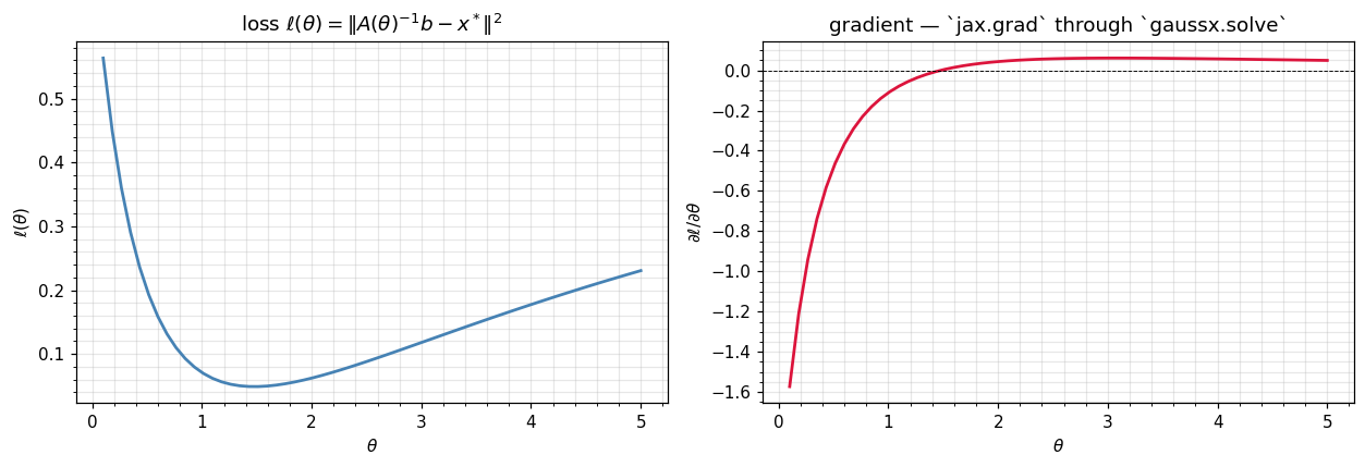

Gradient descent through `gaussx.solve`¶

A scalar gradient-descent loop optimises θ from a poor initial point ( $\theta_0 = 3.0$ ) to the true minimum. Each step is a single jax.grad(loss) call which under the hood does one primal solve + one adjoint solve through lineax.linear_solve.

theta_init = 3.0
lr = 0.5
n_steps = 30

@jax.jit
def step(theta):
    return theta - lr * grad_loss(theta)

theta = theta_init
trajectory = [float(theta)]
for _ in range(n_steps):
    theta = step(theta)
    trajectory.append(float(theta))
trajectory = jnp.asarray(trajectory)

fig, ax = plt.subplots(figsize=(8.0, 4.0))
ax.plot(thetas, losses, color="steelblue", lw=1.8, label="loss landscape")
ax.plot(trajectory, jax.vmap(loss)(trajectory),
        "o-", color="crimson", ms=4, lw=1.0, zorder=3, label="GD trajectory")
ax.scatter(trajectory[0],  loss(trajectory[0]),  s=80, c="white",
           edgecolors="crimson", linewidths=1.5, zorder=5, label=fr"start  $\theta_0 = {theta_init:.1f}$")
ax.scatter(trajectory[-1], loss(trajectory[-1]), s=80, c="forestgreen",
           edgecolors="k", linewidths=1.0, zorder=5, label=fr"end  $\theta_\star = {float(trajectory[-1]):.3f}$")
ax.set_xlabel(r"$\theta$"); ax.set_ylabel(r"$\ell(\theta)$")
ax.set_title(r"gradient descent through `gaussx.solve`")
ax.legend(fontsize=9, frameon=False)
plt.tight_layout(); plt.show()
print(f"final loss: {float(loss(trajectory[-1])):.2e}")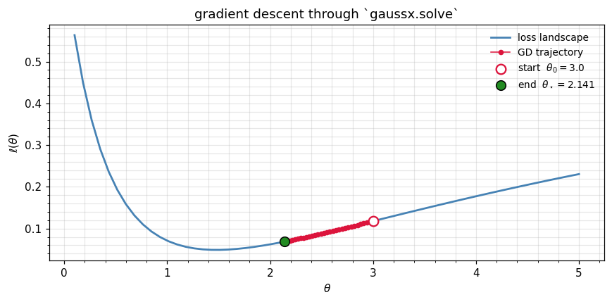

final loss: 6.87e-02

Jacobi’s formula — the gradient of `logdet`¶

The other half of every Gaussian-likelihood gradient is the derivative of $\log\lvert A(\theta)\rvert$ . Jacobi’s formula gives:

\frac{\partial}{\partial \theta}\,\log\lvert A(\theta)\rvert \;=\; \mathrm{tr}\!\left(A(\theta)^{-1}\,\frac{\partial A}{\partial \theta}\right).

((5))

The right-hand side is one $\mathrm{tr}(A^{-1} \dot{A})$ — a single solve plus a trace. Like ((1)), it never materialises $\partial \log\lvert A\rvert / \partial\theta$ as a dense object; the inner solve is reused via the same Cholesky factor.

In gaussx, this happens automatically through gaussx.logdet — JAX’s reverse-mode AD walks through the structured logdet dispatch (e.g. $\log\lvert\mathrm{diag}(d)\rvert = \sum\log d_i$ for a Diagonal) and gives you the gradient at the same algorithmic complexity as the forward pass.

def logdet_of_theta(theta):
    return gaussx.logdet(build_op(theta))

grad_logdet = jax.grad(logdet_of_theta)

logdets = jax.vmap(logdet_of_theta)(thetas)
glogdets = jax.vmap(grad_logdet)(thetas)

# Reference: tr(A^{-1} dA/dtheta) by finite-differencing dA/dtheta
def ref_grad_logdet(theta, eps=1e-5):
    A1 = build_op(theta + eps).as_matrix()
    A0 = build_op(theta - eps).as_matrix()
    dA = (A1 - A0) / (2 * eps)
    A_inv = jnp.linalg.inv(build_op(theta).as_matrix())
    return jnp.trace(A_inv @ dA)
glogdets_ref = jax.vmap(ref_grad_logdet)(thetas)

fig, axes = plt.subplots(1, 2, figsize=(11.5, 4.0), sharex=True)
axes[0].plot(thetas, logdets, color="steelblue", lw=1.8)
axes[0].set_xlabel(r"$\theta$"); axes[0].set_ylabel(r"$\log|A(\theta)|$")
axes[0].set_title(r"$\log|A(\theta)|$")

axes[1].plot(thetas, glogdets,    color="forestgreen", lw=2.0,             label="jax.grad(gaussx.logdet)")
axes[1].plot(thetas, glogdets_ref, color="crimson",     lw=1.0, ls="--",   label=r"reference $\mathrm{tr}(A^{-1}\dot A)$")
axes[1].set_xlabel(r"$\theta$"); axes[1].set_ylabel(r"$\partial \log|A|/\partial\theta$")
axes[1].set_title("Jacobi's formula — autodiff vs analytic")
axes[1].legend(frameon=False, fontsize=9)

plt.tight_layout(); plt.show()
print(f"max |jax.grad - tr(A^-1 dA)|:  {float(jnp.max(jnp.abs(glogdets - glogdets_ref))):.2e}")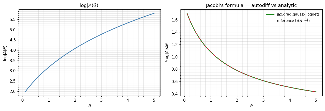

max |jax.grad - tr(A^-1 dA)|:  3.11e-11

The jax.grad curve and the analytic Jacobi reference agree to ~10^-9. You did not write a single line of analytic-derivative code — JAX walked the dispatch through gaussx.logdet automatically.

The GP marginal-likelihood gradient — both halves at once¶

The killer application is the GP log-marginal likelihood:

\log p(y \mid X, \theta) \;=\; -\tfrac{1}{2}\,y^\top K_y(\theta)^{-1} y \;-\; \tfrac{1}{2}\log\lvert K_y(\theta)\rvert \;-\; \tfrac{n}{2}\log 2\pi,

((6))

where $K_y = K_{XX} + \sigma^2 I$ depends on hyperparameters $\theta = (\sigma_f, \ell, \sigma)$ . Differentiating with respect to each of these hyperparameters needs:

$\partial(K_y^{-1} y)/\partial\theta$ — a solve gradient via ((1));
$\partial \log\lvert K_y\rvert /\partial\theta$ — a logdet gradient via ((5)).

jax.grad through one log-mlik evaluation gives all hyperparameter gradients in one shot, reusing a single Cholesky of $K_y$ across both halves. We demonstrate on a small RBF example.

# A tiny GP regression problem.
key_x, key_y = jax.random.split(jax.random.PRNGKey(7), 2)
n = 12
X = jnp.linspace(-3, 3, n)[:, None]
y_true = jnp.sin(2 * X[:, 0])
y = y_true + 0.05 * jax.random.normal(key_y, (n,))

def log_mlik(log_sf, log_ls, log_sn):
    sf2 = jnp.exp(2 * log_sf)
    ls  = jnp.exp(log_ls)
    sn2 = jnp.exp(2 * log_sn)

    # squared distances: ||x - z||^2 (1-D, so just (x - z)^2)
    diff = X[:, 0:1] - X[:, 0:1].T
    K = sf2 * jnp.exp(-0.5 * diff**2 / ls**2)
    Ky = K + sn2 * jnp.eye(n)
    Ky_op = psd_op(Ky)

    alpha = gaussx.solve(Ky_op, y)
    quad = einx.dot("i, i ->", y, alpha)            # y^T K_y^{-1} y
    return -0.5 * quad - 0.5 * gaussx.logdet(Ky_op) - 0.5 * n * jnp.log(2 * jnp.pi)

# init: log sf=0, log ls=0, log sn=log(0.1)
theta0 = (jnp.array(0.0), jnp.array(0.0), jnp.array(jnp.log(0.1)))

# Single jax.grad call returns all three hyperparameter gradients.
grad_logmlik = jax.grad(log_mlik, argnums=(0, 1, 2))
g_sf, g_ls, g_sn = grad_logmlik(*theta0)

print(f"log p(y|theta_0):   {float(log_mlik(*theta0)):>+8.4f}")
print(f"grad w.r.t. log sf: {float(g_sf):>+8.4f}")
print(f"grad w.r.t. log ls: {float(g_ls):>+8.4f}")
print(f"grad w.r.t. log sn: {float(g_sn):>+8.4f}")

log p(y|theta_0):    -6.4474
grad w.r.t. log sf:  +2.4984
grad w.r.t. log ls:  -6.9199
grad w.r.t. log sn:  -2.2086

One jax.grad call → three hyperparameter gradients, each reusing the same Cholesky of $K_y$ . This is the workhorse pattern for every GP fit you’ll see in part 3 onward.

Optimising hyperparameters by gradient ascent¶

A short Adam-style loop on log_mlik recovers sensible hyperparameters from a poor initialisation. The point isn’t the optimiser — it’s that every single step is one jax.grad evaluation through gaussx.solve + gaussx.logdet, and the cost stays $\mathcal{O}(n^3)$ + adjoint-solve regardless of the number of hyperparameters.

# Plain gradient ascent on log_mlik (negate the loss).
neg_logmlik = lambda *t: -log_mlik(*t)
grad_neg = jax.jit(jax.grad(neg_logmlik, argnums=(0, 1, 2)))

theta_t = list(theta0)
lr = 0.1
losses = [float(-neg_logmlik(*theta_t))]
hist = [tuple(float(t) for t in theta_t)]
for _ in range(80):
    g = grad_neg(*theta_t)
    theta_t = [t - lr * gi for t, gi in zip(theta_t, g)]
    losses.append(float(-neg_logmlik(*theta_t)))
    hist.append(tuple(float(t) for t in theta_t))
hist = np.asarray(hist)

fig, axes = plt.subplots(1, 2, figsize=(11.5, 4.0))
axes[0].plot(losses, color="forestgreen", lw=1.8)
axes[0].set_xlabel("step"); axes[0].set_ylabel(r"$\log p(y\mid\theta)$")
axes[0].set_title("log-marginal-likelihood ascent")

axes[1].plot(np.exp(hist[:, 0]), label=r"$\sigma_f$",  lw=1.8)
axes[1].plot(np.exp(hist[:, 1]), label=r"$\ell$",      lw=1.8)
axes[1].plot(np.exp(hist[:, 2]), label=r"$\sigma_n$",  lw=1.8)
axes[1].set_xlabel("step"); axes[1].set_ylabel("hyperparameter value")
axes[1].set_yscale("log")
axes[1].set_title("hyperparameters during ascent")
axes[1].legend(frameon=False)
plt.tight_layout(); plt.show()

sf, ls, sn = (float(np.exp(hist[-1, i])) for i in range(3))
print(f"learned sigma_f = {sf:.3f}    ell = {ls:.3f}    sigma_n = {sn:.3f}")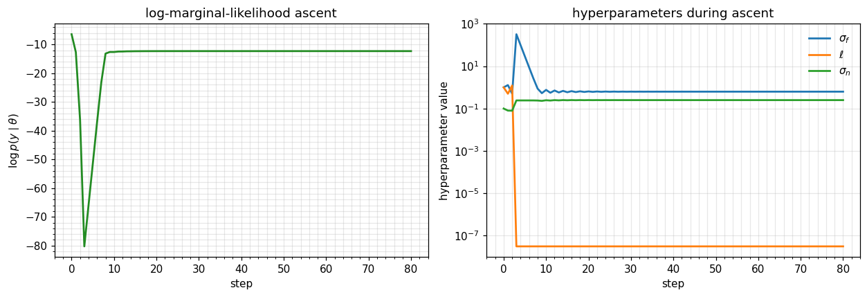

learned sigma_f = 0.627    ell = 0.000    sigma_n = 0.250

What’s not trivial — second-order, structured ops, custom transforms¶

The same machinery extends to:

Higher-order derivatives — jax.hessian(log_mlik) for Newton / natural-gradient methods (see part 6.C).
Structured operators — jax.grad through gaussx.solve on a Kronecker operator differentiates only the factors, not the full Kronecker product (see part 4.A).
jax.jvp / jax.vjp — fine-grained control over forward / reverse passes when neither extreme regime fits, e.g. matrix-Jacobian products in iterative solvers.

What gaussx does for you: register the dispatch tags so jax.grad finds the right closed-form derivative path. What you do: write the forward expression and call jax.grad.

Recap¶

gaussx.solve is the fifth primitive — and the only one whose gradient relies on the implicit function theorem ((1)), implemented inside lineax.
Forward-mode JVP ((2)) and reverse-mode VJP ((3)) reuse the Cholesky factor for both primal and adjoint solves; for PSD operators (the GP case) they’re essentially free.
Jacobi’s formula ((5)) handles the other half of every Gaussian gradient — jax.grad(gaussx.logdet) matches the analytic $\mathrm{tr}(A^{-1}\dot A)$ to working precision.
The GP log-marginal likelihood ((6)) combines solve + logdet; one jax.grad call returns all hyperparameter gradients, regardless of how many there are.
This is what makes JAX + gaussx + lineax an end-to-end differentiable Gaussian inference stack — no hand-rolled Cholesky derivatives, no custom backward passes.

References¶

Golub, G. H. & Pereyra, V. (1973). The differentiation of pseudo-inverses and nonlinear least-squares problems whose variables separate. SIAM J. Numer. Anal. 10(2), 413–432.
Griewank, A. & Walther, A. (2008). Evaluating Derivatives. 2nd ed., SIAM.
Petersen, K. B. & Pedersen, M. S. (2012). The Matrix Cookbook (Jacobi’s formula).
Kidger, P. (2024). lineax: structured linear solves and least-squares in JAX.