Structured MVN sampling dispatch — keeping the root cheap
Sampling from via the reparameterisation trick (already met as ((5))) is
The matrix is any root of Σ. The cheapest choice depends on what Σ looks like:
| Σ structure | Best root | Cost (square ) |
|---|---|---|
| Dense | Cholesky | |
| Diagonal | — element-wise | |
| Kronecker | instead of | |
| Block-diagonal | ||
| Block-tridiagonal precision Λ (Markov chain) | Banded Cholesky + triangular solve | instead of |
| Low-rank update | No closed-form root; sample as two independent draws | varies |
| Toeplitz / KroneckerSum / SumKronecker | Falls back to dense in gaussx today; smart routes (FFT / eigen / Lanczos) are listed in §9 below | until wired |
This is exactly what gaussx.cholesky and gaussx.sqrt do — dispatch on operator type and return a structured root operator of the same family. Sampling stays cheap automatically.
This notebook walks the dispatch table:
- dense baseline (((5)) recap with
gaussx.cholesky), - diagonal — element-wise sqrt, the simplest dispatch,
- Kronecker root identity + Monte-Carlo cross-check,
- BlockDiag root identity + per-block parallelism,
- BlockTriDiag → LowerBlockTriDiag — banded Cholesky for Markov-chain precisions,
- low-rank update — what gaussx does when there’s no closed-form root,
- Cholesky vs symmetric square root (when each one is the right answer),
- timing: structured roots scale with the factor size, not the product,
- operators that currently fall back to dense (Toeplitz / KroneckerSum / SumKronecker) and what their smart roots would be.
Prerequisites: 0.1 — Multivariate Gaussian (especially ((5)) and ((4))), 0.2 — MultivariateNormal API.
from __future__ import annotations

import time
import warnings
warnings.filterwarnings("ignore", message=r".*IProgress.*")

import einx
import jax
import jax.numpy as jnp
import lineax as lx
import matplotlib.pyplot as plt
import numpy as np
import gaussx
from gaussx import (
    BlockDiag,
    Kronecker,
    LowRankUpdate,
    MultivariateNormal,
    cholesky,
    sqrt as op_sqrt,
)

jax.config.update("jax_enable_x64", True)
KEY = jax.random.PRNGKey(0)
plt.rcParams.update({
    "figure.dpi": 110,
    "axes.grid": True,
    "axes.grid.which": "both",
    "xtick.minor.visible": True,
    "ytick.minor.visible": True,
    "grid.alpha": 0.3,
})


def psd_op(M):
    return lx.MatrixLinearOperator(M, lx.positive_semidefinite_tag)
Sampling = a single matvec against any root¶
Once you have a root with , drawing samples is a matmul:
gaussx.cholesky(Sigma_op) returns a structured operator of the same family as Σ. Multiplying noise through via mv (or composed Kronecker/BlockDiag ops) keeps the structure all the way down — you never materialise the dense .
1. Dense baseline¶
For an arbitrary SPD Σ the standard recipe is the Cholesky factor:
gaussx.cholesky on a MatrixLinearOperator returns the dense Cholesky as a new MatrixLinearOperator.
n = 6
key, k_M, k_eps = jax.random.split(KEY, 3)
M = jax.random.normal(k_M, (n, n))
Sigma_dense = M @ M.T + 0.5 * jnp.eye(n)
Sigma_op    = psd_op(Sigma_dense)

L_op = cholesky(Sigma_op)
L    = L_op.as_matrix()
print("L type :", type(L_op).__name__)
print("L L^T - Sigma  ||F  =",
      f"{float(jnp.linalg.norm(L @ L.T - Sigma_dense)):.2e}")

# Sample 50000 draws and compare empirical covariance.
S = 50_000
mu = jnp.zeros(n)
eps = jax.random.normal(k_eps, (S, n))
X = mu + einx.dot("s a, b a -> s b", eps, L)
Sigma_emp = einx.dot("s i, s j -> i j", X, X) / S

print("dense  ||Sigma_emp - Sigma||_F  =",
      f"{float(jnp.linalg.norm(Sigma_emp - Sigma_dense)):.2e}    "
      f"(MC noise ~ ||Sigma||_F * n / sqrt(S))")
L type : MatrixLinearOperator
L L^T - Sigma ||F = 2.53e-15
dense ||Sigma_emp - Sigma||_F = 1.39e-01 (MC noise ~ ||Sigma||_F * n / sqrt(S))
2. Diagonal — the simplest dispatch¶
When , the Cholesky is element-wise:
gaussx.cholesky(DiagonalLinearOperator(d)) returns another DiagonalLinearOperator — no matrix is ever materialised. Sampling is one element-wise multiply.
This is the structural foundation of mean-field variational inference (where Σ is constrained diagonal by design) and of factorised Gaussian priors.
key, k_eps = jax.random.split(KEY)
n_diag = 8
diag_var = jnp.array([4.0, 1.0, 9.0, 0.25, 2.5, 0.5, 16.0, 1.5])
D_op = lx.DiagonalLinearOperator(diag_var)

L_D = cholesky(D_op)
print("L type :", type(L_D).__name__)
print("L diag :", np.asarray(L_D.diagonal))
print("L diag = sqrt(var)?", bool(jnp.allclose(L_D.diagonal, jnp.sqrt(diag_var))))

# Sample 50000 draws -- one element-wise multiply per draw.
S = 50_000
eps = jax.random.normal(k_eps, (S, n_diag))
X = jax.vmap(L_D.mv)(eps)
diag_emp = einx.var("s d -> d", X)
print("\nempirical diag(Sigma):", np.asarray(diag_emp))
print("true diag(Sigma)     :", np.asarray(diag_var))
print(f"max relative error    = {float(jnp.max(jnp.abs(diag_emp - diag_var) / diag_var)):.2e}")
L type : DiagonalLinearOperator
L diag : [2. 1. 3. 0.5 1.58113883 0.70710678
4. 1.22474487]
L diag = sqrt(var)? True
empirical diag(Sigma): [ 4.02239356  0.99896439  8.97460525  0.25057673  2.50498229  0.49966097
 15.99077588  1.51320825]
true diag(Sigma)     : [ 4.    1.    9.    0.25  2.5   0.5  16.    1.5 ]
max relative error    = 8.81e-03
3. Kronecker — the canonical dispatch win¶
For SPD and ,
So instead of factorising the Kronecker product, factorise the two small blocks and Kronecker their Choleskys. gaussx.cholesky(Kronecker(A_op, B_op)) does exactly this and returns another Kronecker — sampling stays instead of .
n_A, n_B = 4, 5
key, k_A, k_B, k_eps = jax.random.split(KEY, 4)

MA = jax.random.normal(k_A, (n_A, n_A))
A  = MA @ MA.T + 0.3 * jnp.eye(n_A)
MB = jax.random.normal(k_B, (n_B, n_B))
B  = MB @ MB.T + 0.3 * jnp.eye(n_B)

A_op = psd_op(A); B_op = psd_op(B)
K_op = Kronecker(A_op, B_op)

L_K  = cholesky(K_op)
print("L type            :", type(L_K).__name__)
print("L_K factor types  :", [type(o).__name__ for o in L_K.operators])

# Sanity: chol(A) ⊗ chol(B) really is the Cholesky of A ⊗ B.
LA = jnp.linalg.cholesky(A); LB = jnp.linalg.cholesky(B)
LK_dense_ref = jnp.kron(LA, LB)
print("\nL_K - chol(A) ⊗ chol(B)  ||F  =",
      f"{float(jnp.linalg.norm(L_K.as_matrix() - LK_dense_ref)):.2e}")

# Sample via the *structured* Kronecker root: each draw is a matvec on the
# small factors -- never instantiate the (n_A n_B) x (n_A n_B) matrix.
S = 80_000
n = n_A * n_B
eps = jax.random.normal(k_eps, (S, n))
X = jax.vmap(L_K.mv)(eps)
Sigma_emp = einx.dot("s i, s j -> i j", X, X) / S
Sigma_true = jnp.kron(A, B)
print(f"||Sigma_emp - kron(A,B)||_F  = "
      f"{float(jnp.linalg.norm(Sigma_emp - Sigma_true)):.2e}    "
      f"(MC noise ~ ||Sigma||_F * n / sqrt(S))")
L type : Kronecker
L_K factor types : ['MatrixLinearOperator', 'MatrixLinearOperator']
L_K - chol(A) ⊗ chol(B) ||F = 0.00e+00
||Sigma_emp - kron(A,B)||_F = 9.84e-01 (MC noise ~ ||Sigma||_F * n / sqrt(S))
4. Block-diagonal — embarrassingly parallel¶
Each block factorises independently — perfect for vmap if all have the same shape, or for jax.tree_map if they don’t. gaussx.cholesky(BlockDiag(...)) returns another BlockDiag whose constituents are the per-block Choleskys.
key, k_C, k_D, k_E, k_eps = jax.random.split(KEY, 5)
def make_psd(key, k):
    M = jax.random.normal(key, (k, k))
    return psd_op(M @ M.T + 0.3 * jnp.eye(k))

C_op = make_psd(k_C, 3)
D_op = make_psd(k_D, 4)
E_op = make_psd(k_E, 2)
BD_op = BlockDiag(C_op, D_op, E_op)

L_BD = cholesky(BD_op)
print("L type         :", type(L_BD).__name__)
print("inner blocks   :", [type(b).__name__ for b in L_BD.operators])

# Per-block reference Choleskys
LC = jnp.linalg.cholesky(C_op.as_matrix())
LD = jnp.linalg.cholesky(D_op.as_matrix())
LE = jnp.linalg.cholesky(E_op.as_matrix())

block_errs = [
    float(jnp.linalg.norm(L_BD.operators[k].as_matrix() - L_ref))
    for k, L_ref in enumerate([LC, LD, LE])
]
print("per-block ||L_dispatch - L_ref||_F:", [f"{e:.2e}" for e in block_errs])

# Monte-Carlo sample-covariance check
S = 60_000
n_total = 3 + 4 + 2
eps = jax.random.normal(k_eps, (S, n_total))
X   = jax.vmap(L_BD.mv)(eps)
Sigma_emp = einx.dot("s i, s j -> i j", X, X) / S
Sigma_true = jax.scipy.linalg.block_diag(C_op.as_matrix(), D_op.as_matrix(), E_op.as_matrix())
print(f"\n||Sigma_emp - block-diag||_F  = "
      f"{float(jnp.linalg.norm(Sigma_emp - Sigma_true)):.2e}    "
      f"(MC noise ~ ||Sigma||_F * n / sqrt(S))")
L type : BlockDiag
inner blocks : ['MatrixLinearOperator', 'MatrixLinearOperator', 'MatrixLinearOperator']
per-block ||L_dispatch - L_ref||_F: ['0.00e+00', '0.00e+00', '0.00e+00']
||Sigma_emp - block-diag||_F = 1.59e-01 (MC noise ~ ||Sigma||_F * n / sqrt(S))
5. Block-tridiagonal precision — banded Cholesky + triangular solve¶
A block-tridiagonal precision Λ is the natural representation of a Markov chain over blocks of size — only adjacent time steps interact, so all but the main and one off-diagonal block are zero. Its Cholesky factor is itself block-bidiagonal:
gaussx.cholesky(BlockTriDiag(diag_blocks, sub_blocks)) returns a LowerBlockTriDiag operator whose mv and triangular solve both run in instead of .
Sampling from — the actual Markov-chain marginal — does not multiply by (that would give a draw from , not ). The correct recipe is the triangular back-solve
executed via gaussx.solve(L.T, eps). Because is block-bidiagonal, this back-solve runs in — the same cost class as the matvec, never materialising (which would be dense). This is the workhorse for state-space / Markov-GP posterior sampling: the precision of in a linear-Gaussian SSM is block-tridiagonal by construction, and Σ is dense, so we sample by never inverting Λ explicitly.
from gaussx import solve as gx_solve

N_blk, d_blk = 12, 3
key, k_eps = jax.random.split(KEY)

# Build a random SPD block-tridiagonal *precision* Lambda: diag blocks SPD,
# sub-diagonal blocks small enough that the whole matrix is SPD.
key, k_diag, k_sub = jax.random.split(key, 3)
diag_raw = jax.random.normal(k_diag, (N_blk, d_blk, d_blk))
diag_blk = einx.dot("n i a, n j a -> n i j", diag_raw, diag_raw) \
         + 3.0 * jnp.broadcast_to(jnp.eye(d_blk), (N_blk, d_blk, d_blk))
sub_blk  = 0.2 * jax.random.normal(k_sub, (N_blk - 1, d_blk, d_blk))

Lambda_op = gaussx.BlockTriDiag(diag_blk, sub_blk, tags=lx.positive_semidefinite_tag)
L_BT      = cholesky(Lambda_op)                          # Lambda = L L^T, L lower block-bidiagonal
print("Lambda type :", type(Lambda_op).__name__)
print("L type      :", type(L_BT).__name__)

# Cholesky round-trip: L L^T = Lambda
L_dense      = L_BT.as_matrix()
Lambda_dense = Lambda_op.as_matrix()
print(f"||L L^T - Lambda||_F  =  {float(jnp.linalg.norm(L_dense @ L_dense.T - Lambda_dense)):.2e}")

# Sampling target: x ~ N(0, Sigma) with Sigma = Lambda^{-1} (the actual Markov
# chain marginal). The recipe from [](#eq:blocktridiag-root) is x = L^{-T} eps,
# which we compute via gaussx.solve(L.T, eps) -- a banded triangular solve in
# O(N d^3), never materialising the dense Sigma.
n = N_blk * d_blk
S = 40_000
eps = jax.random.normal(k_eps, (S, n))
X = jax.vmap(lambda e: gx_solve(L_BT.T, e))(eps)
Sigma_emp = einx.dot("s i, s j -> i j", X, X) / S

# Reference Sigma = Lambda^{-1} (dense, only built here for the cross-check).
Sigma_dense_ref = jnp.linalg.inv(Lambda_dense)
print(f"||Sigma_emp - Lambda^-1||_F  =  "
      f"{float(jnp.linalg.norm(Sigma_emp - Sigma_dense_ref)):.2e}    "
      f"(MC noise ~ ||Sigma||_F * n / sqrt(S))")

# Sanity: multiplying eps by L instead would have given draws from N(0, Lambda),
# not N(0, Lambda^{-1}). Show the difference.
X_wrong = jax.vmap(L_BT.mv)(eps)
Cov_wrong = einx.dot("s i, s j -> i j", X_wrong, X_wrong) / S
print(f"||Cov(L @ eps) - Lambda||_F  =  "
      f"{float(jnp.linalg.norm(Cov_wrong - Lambda_dense)):.2e}    "
      f"(this would be wrong target; matches Lambda, not Lambda^-1)")
Lambda type : BlockTriDiag
L type : LowerBlockTriDiag
||L L^T - Lambda||_F = 5.11e-15
||Sigma_emp - Lambda^-1||_F = 4.05e-02 (MC noise ~ ||Sigma||_F * n / sqrt(S))
||Cov(L @ eps) - Lambda||_F = 1.12e+00 (this would be wrong target; matches Lambda, not Lambda^-1)
6. Low-rank update — when there is no closed-form root¶
For with already factorised as , you can build a sampling root via the whitening trick:
The two noise vectors are independent so . No need for a closed-form Cholesky of the sum — the rank correction stays separate. This is how ensemble Kalman, low-rank GP priors, and rank-revealing covariance estimates sample at scale.
gaussx.cholesky(LowRankUpdate(...)) does not return a structured root for the general case (no closed form), but the additive sampling identity above is straightforward to implement in user code — and the operator stays cheap because and keep their structure.
key, k_U, k_eps0, k_eps1 = jax.random.split(KEY, 4)
n_lr = 6
r    = 2                                # rank of the update

base_M = jax.random.normal(jax.random.PRNGKey(7), (n_lr, n_lr))
Sigma0 = base_M @ base_M.T + 0.4 * jnp.eye(n_lr)
Sigma0_op = psd_op(Sigma0)

U = jax.random.normal(k_U, (n_lr, r))
D = jnp.diag(jnp.array([1.0, 0.5]))     # rank-2 PSD diag
Sigma_full = Sigma0 + einx.dot("i a, a b, j b -> i j", U, D, U)

# Structured sampling: no Cholesky of the sum, just two independent draws.
L0 = jnp.linalg.cholesky(Sigma0)
sqrtD = jnp.sqrt(jnp.diag(D))
S = 80_000
eps0 = jax.random.normal(k_eps0, (S, n_lr))
eps1 = jax.random.normal(k_eps1, (S, r))
X = einx.dot("s a, b a -> s b", eps0, L0) \
  + einx.multiply("s b, b -> s b", eps1, sqrtD) @ U.T

Sigma_emp = einx.dot("s i, s j -> i j", X, X) / S
print(f"||Sigma_emp - (Sigma0 + U D U^T)||_F  = "
      f"{float(jnp.linalg.norm(Sigma_emp - Sigma_full)):.2e}    "
      f"(MC noise ~ ||Sigma||_F * n / sqrt(S))")
||Sigma_emp - (Sigma0 + U D U^T)||_F = 1.25e-01 (MC noise ~ ||Sigma||_F * n / sqrt(S))
7. Cholesky vs symmetric square root¶
There’s more than one root. The symmetric square root satisfies
and is computed via the eigendecomposition (you’ve already seen as ((4))). gaussx.sqrt returns this.
Both (Cholesky) and (symmetric) generate the same Gaussian — but they map a fixed to different points. When does this matter?
- Sampling-only workflows: doesn’t matter. Any root produces correct samples.
- Path-coupled samples (e.g. ((5)) “same noise, three roots”): the choice of root induces correlated draws — useful in QMC, antithetic sampling, and reparameterised gradient estimators where you want the same to produce a “matched pair” across two distributions.
- Numerical stability: Cholesky can fail or amplify error on near-singular Σ; symmetric sqrt is safer (eigendecomposition is more forgiving) but ~3× more expensive.
- Symmetric has the property , which appears in 2-Wasserstein distances between Gaussians — Cholesky doesn’t.
S_op = op_sqrt(Sigma_op)
S_mat = S_op.as_matrix()
print("symmetric: S = S^T?         ",
      bool(jnp.allclose(S_mat, S_mat.T, atol=1e-10)))
print("symmetric: S @ S = Sigma?   ",
      f"{float(jnp.linalg.norm(S_mat @ S_mat - Sigma_dense)):.2e}")
print("Cholesky:  L L^T = Sigma?   ",
      f"{float(jnp.linalg.norm(L @ L.T - Sigma_dense)):.2e}")

# Same noise, two roots -> two correlated point clouds.
n_dense = Sigma_dense.shape[0]
S_n = 4_000
key_, kc = jax.random.split(KEY)
eps_dense = jax.random.normal(kc, (S_n, n_dense))
X_chol = einx.dot("s a, b a -> s b", eps_dense, L)
X_sqrt = einx.dot("s a, b a -> s b", eps_dense, S_mat)

# Their *covariances* match (same Gaussian); their *coordinates* differ.
print("\nSame eps, different roots:")
print(f"  ||cov(X_chol) - cov(X_sqrt)||_F = "
      f"{float(jnp.linalg.norm(jnp.cov(X_chol.T) - jnp.cov(X_sqrt.T))):.2e}")
print(f"  ||X_chol - X_sqrt||_F           = "
      f"{float(jnp.linalg.norm(X_chol - X_sqrt)):.2e}    (large -- different points)")
symmetric: S = S^T? True
symmetric: S @ S = Sigma? 1.49e-14
Cholesky: L L^T = Sigma? 2.53e-15
Same eps, different roots:
  ||cov(X_chol) - cov(X_sqrt)||_F = 6.08e-01
||X_chol - X_sqrt||_F = 2.09e+02 (large -- different points)
8. Timing — when dispatch saves you¶
The Kronecker dispatch is the textbook win: factorise two small matrices instead of one giant one. We compare three sampling pipelines for at growing factor sizes:
- Dense Cholesky: build the full Kronecker product, factorise, sample.
- Structured Cholesky:
gaussx.cholesky(Kronecker(A_op, B_op))— two small Choleskys, lazy product. - Reference: the explicit Kronecker-of-Choleskys identity by hand.
The first scales as ; the second and third scale as .
def time_one(fn, n_runs=10):
    fn().block_until_ready()
    t0 = time.perf_counter()
    for _ in range(n_runs):
        fn().block_until_ready()
    return (time.perf_counter() - t0) / n_runs

sizes = [4, 8, 16, 24, 32]
S = 256
records = {"dense": [], "structured": [], "ref": []}

# Each timed path runs *factorisation + sampling* end-to-end so the speedups
# reflect what you'd actually feel as a user, not just the matvec. The dense
# path's Cholesky is recomputed inside f_dense, so the structured path's
# cholesky is also recomputed inside f_struct (and the explicit Kronecker
# product is rebuilt inside f_ref). Apples to apples.
for n_AB in sizes:
    key, ka, kb, ke = jax.random.split(jax.random.PRNGKey(123 + n_AB), 4)
    MA = jax.random.normal(ka, (n_AB, n_AB))
    A_  = MA @ MA.T + 0.3 * jnp.eye(n_AB)
    MB = jax.random.normal(kb, (n_AB, n_AB))
    B_  = MB @ MB.T + 0.3 * jnp.eye(n_AB)
    A_op_ = psd_op(A_); B_op_ = psd_op(B_)
    K_dense = jnp.kron(A_, B_)
    K_op_   = Kronecker(A_op_, B_op_)
    eps     = jax.random.normal(ke, (S, n_AB * n_AB))

    # 1) Dense path — Cholesky of the full Kronecker product, then sample.
    @jax.jit
    def f_dense():
        L = jnp.linalg.cholesky(K_dense)
        return einx.dot("s a, b a -> s b", eps, L)

    # 2) Structured: gaussx.cholesky returns Kronecker, sample via mv.
    #    Includes the cholesky call inside the timed function so it's
    #    measured the same way as f_dense above.
    @jax.jit
    def f_struct():
        L = cholesky(K_op_)
        return jax.vmap(L.mv)(eps)

    # 3) Reference: explicit kron of small Choleskys (factor + sample).
    @jax.jit
    def f_ref():
        LA_ = jnp.linalg.cholesky(A_); LB_ = jnp.linalg.cholesky(B_)
        L_kron = jnp.kron(LA_, LB_)
        return einx.dot("s a, b a -> s b", eps, L_kron)

    records["dense"     ].append(time_one(f_dense))
    records["structured"].append(time_one(f_struct))
    records["ref"       ].append(time_one(f_ref))

records = {k: np.asarray(v) for k, v in records.items()}
ns = np.array(sizes)
print(f"{'n_A=n_B':>8s} {'dense (s)':>12s} {'struct (s)':>12s} {'ref (s)':>10s}  speedup")
for i, n_AB in enumerate(sizes):
    sp = records["dense"][i] / records["structured"][i]
    print(f"{n_AB:>8d} {records['dense'][i]:>12.4f} {records['structured'][i]:>12.4f} "
          f"{records['ref'][i]:>10.4f}   {sp:>5.1f}x")
n_A=n_B dense (s) struct (s) ref (s) speedup
4 0.0001 0.0001 0.0000 1.2x
8 0.0001 0.0002 0.0001 1.0x
16 0.0010 0.0006 0.0005 1.7x
24 0.0037 0.0010 0.0011 3.7x
32 0.4464 0.0017 0.0029 269.7x
fig, ax = plt.subplots(figsize=(7.0, 4.0))
ax.plot(ns, records["dense"],      "o-", color="crimson",   lw=1.8, label=r"dense $(n_A n_B)^3$")
ax.plot(ns, records["structured"], "s-", color="steelblue", lw=1.8, label=r"gaussx.cholesky(Kronecker)")
ax.plot(ns, records["ref"],        "^-", color="forestgreen", lw=1.6, label=r"explicit chol(A) $\otimes$ chol(B)")
ax.set_xscale("log"); ax.set_yscale("log")
ax.set_xlabel(r"$n_A = n_B$  (so total size $= n_A n_B$)")
ax.set_ylabel("seconds per sample batch (S=256)")
ax.set_title("Kronecker dispatch keeps sampling cheap")
ax.legend(frameon=False, fontsize=8)
plt.tight_layout(); plt.show()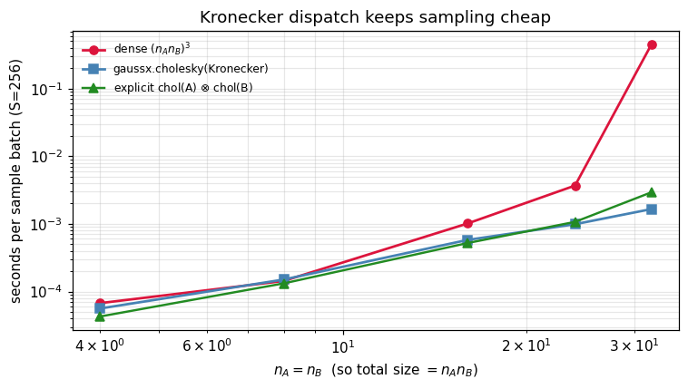
What doesn’t dispatch yet¶
A few operators in gaussx currently have no closed-form structured Cholesky and fall back to materialising the matrix and calling jnp.linalg.cholesky. Each has a known smarter route — listing them here as future work and as a reminder that gaussx.cholesky(op) always returns something correct, just not always something cheap.
| Operator | Smart route (not yet wired) | Reference |
|---|---|---|
Toeplitz () | Circulant embedding + FFT — sampling for stationary 1D processes | Wood & Chan (1994), J. Comp. Graph. Stat.; gaussx#168 |
KroneckerSum () | Eigendecomposition: , | Saatçi (2011), thesis; gaussx#169 |
SumKronecker () | Conjugate-gradient + matfree Lanczos for | Pleiss et al. (2018), GPyTorch; gaussx#170 |
For now, on these operators gaussx.cholesky produces a dense MatrixLinearOperator and you sample as in section 1 (the dispatch path is just slower than it could be). The three tracking issues above carry full math + proposed APIs.
Where the dispatch wins¶
| Setting | Σ structure | Root used | Why |
|---|---|---|---|
| Mean-field VI / factorised priors | Diagonal | ((4)) | Element-wise sqrt — no matrix anywhere |
| Spatio-temporal GPs (separable) | ((5)) | Two small Choleskys instead of one | |
| Independent ensembles / multi-output GPs | BlockDiag() | ((6)) | Embarrassingly parallel per output |
| State-space / Markov GPs (part 7) | Λ block-tridiagonal | ((8)) | Banded Cholesky → posterior sampling |
| Ensemble Kalman / low-rank GP priors | ((9)) | Sample — never factorise the sum | |
| 2-Wasserstein / OT between Gaussians | symmetric sqrt | ((10)) | Closed-form uses |
| Antithetic / coupled sampling | any deterministic root | ((1)) | Same across two distributions ⇒ correlated estimators |
| Reparameterised VI gradients | Cholesky | ((5)) | propagates cleanly through jax.grad |
Recap¶
- Sampling = matvec against any root of Σ (((1))). gaussx exposes both Cholesky and symmetric sqrt; structured operators get structured roots.
- (((5))) and (((6))) are both built into
gaussx.cholesky. - Low-rank updates avoid the closed-form root by injecting the rank correction as a second independent draw (((9))).
- Symmetric (((10))) is the right choice for 2-Wasserstein, antithetic sampling, and any setting that wants .
References¶
- Rasmussen, C. E. & Williams, C. K. I. (2006). Gaussian Processes for Machine Learning. MIT Press, App. A.4.
- Saatçi, Y. (2011). Scalable Inference for Structured Gaussian Process Models. PhD thesis, Cambridge.
- Higham, N. J. (2008). Functions of Matrices: Theory and Computation. SIAM. (Symmetric square roots.)
- Kingma, D. P. & Welling, M. (2014). Auto-encoding variational Bayes. ICLR. (Reparameterisation trick.)