import autoroot  # noqa: F401, I001
import jax
import jax.numpy as jnp
import jax.random as jrandom
import matplotlib.pyplot as plt
import seaborn as sns
import diffrax as dfx
import xarray as xr
import numpy as np
import functools as ft

from jaxsw._src.models.lorenz96t import L96TParams, L96TState, rhs_lorenz_96t, Lorenz96t

sns.reset_defaults()
sns.set_context(context="talk", font_scale=0.7)
%matplotlib inline
%load_ext autoreload
%autoreload 2
Lorenz 96
- Equation of Motion
- Observation Operator
- Integrate
F = 18.0  # forcing term
b = 10.0  # coupling coefficient
h = 1.0  # ratio of amplitudes
c = 10.0  # time-scale ratio
# initialize state
ndims = 36, 10
noise = (0.01, 0.0)
key = jrandom.PRNGKey(42)
state = L96TState.init_state(ndims=ndims, noise=noise, key=key)
# rhs
x = state.x
y = state.y
assert x.shape == (ndims[0],)
assert y.shape == (ndims[1] * ndims[0],)
x_dot, y_dot, coupling_term = rhs_lorenz_96t(x=x, y=y, F=F, h=h, c=c, b=b)
assert x_dot.shape == x.shape
assert y_dot.shape == y.shape
assert coupling_term.shape == x.shapeModel
K = ndims[0]
J = ndims[1]


def s(k, K):
    """A non-dimension coordinate from -1..+1 corresponding to k=0..K"""
    return 2 * (0.5 + k) / K - 1


k = np.arange(K)  # For coordinate in plots
j = np.arange(J * K)  # For coordinate in plots

# Initial conditions
X_init = s(k, K) * (s(k, K) - 1) * (s(k, K) + 1)
Y_init = 0 * s(j, J * K) * (s(j, J * K) - 1) * (s(j, J * K) + 1)
state_init = L96TState(x=jnp.asarray(X_init), y=jnp.asarray(Y_init))
params = L96TParams(F=F, h=h, b=b, c=c)# # t0 = 0.0
# # t1 = 30.0
# # initialize state
# F = 18.0 # forcing term
# b = 10.0 # coupling coefficient
# h = 1.0 # ratio of amplitudes
# c = 10.0 # time-scale ratio
# ndims = 36, 10
# noise = (0.05, 0.0)
# batchsize = 1
# state_init, params = L96TState.init_state_and_params(
# ndims=ndims, noise=noise, batchsize=batchsize,
# F=F, h=h, b=b, c=c
# )# initialize model
advection = True
l96t_model = Lorenz96t(advection=advection)
# step through
state_dot = l96t_model.equation_of_motion(t=0, state=state_init, args=params)
# state_dot.x.shape
assert state_dot.x.shape == state_init.x.shape
assert state_dot.y.shape == state_init.y.shapeTime Stepping
dt = 0.005
t0 = 0.0
t1 = 2_000

ts = jnp.arange(t0, t1, 1) * dt

saveat = dfx.SaveAt(ts=ts)
saveat
SaveAt(
subs=SubSaveAt(
t0=False,
t1=False,
ts=f32[2000],
steps=False,
fn=<function save_y>
),
dense=False,
solver_state=False,
controller_state=False,
made_jump=False
)# Euler, Constant StepSize
solver = dfx.Tsit5()
stepsize_controller = dfx.PIDController(rtol=1e-5, atol=1e-5)
# integration
sol = dfx.diffeqsolve(
terms=dfx.ODETerm(l96t_model.equation_of_motion),
solver=solver,
t0=ts.min(),
t1=ts.max(),
dt0=dt,
y0=state_init,
saveat=saveat,
args=params,
stepsize_controller=stepsize_controller,
)Analysis
ds_sol = xr.Dataset(
    {
        "x": (("time", "Dx"), sol.ys.x.squeeze()),
        "y": (("time", "Dy"), sol.ys.y.squeeze()),
    },
    coords={
        "time": (["time"], sol.ts.squeeze()),
        "Dx": (["Dx"], np.arange(0, ndims[0])),
        "Dy": (["Dy"], np.arange(np.prod(ndims)) / ndims[1]),
    },
    attrs={
        "ode": "lorenz_96_2layer",
        # "sigma": params.sigma,
        # "beta": params.beta,
        # "rho": params.rho,
    },
)
ds_sol
Loading...
fig, ax = plt.subplots(nrows=2, figsize=(5, 8))

time_step = -1
ds_sol.x.isel(time=time_step).plot(
    ax=ax[0], label="$X_k(t=n_t dt)$", color="tab:orange"
)
ds_sol.x.isel(time=0).plot(
    ax=ax[0], label="$X_k(t=0)$", color="black", linestyle=":", zorder=3
)
ds_sol.y.isel(time=time_step).plot(
    ax=ax[0], label="$Y_{j,k}(t=n_t dt)$", color="tab:green"
)
ds_sol.y.isel(time=0).plot(
    ax=ax[0], label="$Y_{j,k}(t=0)$", color="tab:red", linestyle=":", zorder=3
)
ax[0].legend()
# ax[0].set_ylabel("Time")
ax[0].set_xlabel("k, k + j/J")


# ds_sol.y.plot.contourf(ax=ax[1], cmap="viridis")
# ax[1].set_ylabel("Time")
# ax[1].set_xlabel("Dimension")

plt.tight_layout()
plt.show()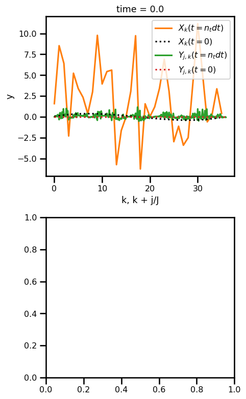
fig, ax = plt.subplots(nrows=2, figsize=(5, 6))

ds_sol.x.plot.contourf(ax=ax[0], cmap="viridis")
ax[0].set_ylabel("Time")
ax[0].set_xlabel("Dimension")


ds_sol.y.plot.contourf(ax=ax[1], cmap="viridis")
ax[1].set_ylabel("Time")
ax[1].set_xlabel("Dimension")

plt.tight_layout()
plt.show()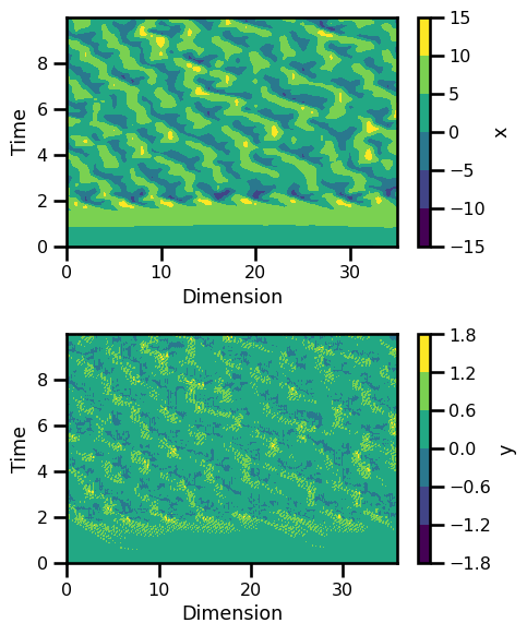
Batch of Trajectories
F = 18.0  # forcing term
b = 10.0  # coupling coefficient
h = 1.0  # ratio of amplitudes
c = 10.0  # time-scale ratio

params = L96TParams(F=F, h=h, b=b, c=c)
# initialize state
ndims = 36, 10
noise = 0.001
batchsize = 50
state = L96TState.init_state(ndims=ndims, noise=noise, batchsize=batchsize)
# rhs
x = state.x
y = state.y
rhs_fn = ft.partial(rhs_lorenz_96t, F=F, h=h, c=c, b=b)
fn_batched = jax.vmap(rhs_fn, in_axes=(0, 0))
x_dot, y_dot, _ = fn_batched(state.x, state.y)
assert x_dot.shape == state.x.shape
assert y_dot.shape == state.y.shapekey = jrandom.PRNGKey(123)
keyx, keyy = jrandom.split(key=key, num=2)
X_init_batch = X_init + noise * jrandom.normal(key=keyx, shape=(batchsize, 1))
Y_init_batch = Y_init + noise * jrandom.normal(key=keyy, shape=(batchsize, 1))
state_init = L96TState(x=jnp.asarray(X_init_batch), y=jnp.asarray(Y_init_batch))
params = L96TParams(F=F, h=h, b=b, c=c)
X_init_batch.shape, X_init.shape, Y_init_batch.shape, Y_init.shape((50, 36), (36,), (50, 360), (360,))# Euler, Constant StepSize
solver = dfx.Tsit5()
stepsize_controller = dfx.ConstantStepSize()
# integration
integrate = lambda state: dfx.diffeqsolve(
terms=dfx.ODETerm(l96t_model.equation_of_motion),
solver=solver,
t0=ts.min(),
t1=ts.max(),
dt0=dt,
y0=state,
saveat=saveat,
args=params,
stepsize_controller=stepsize_controller,
)
sol = jax.vmap(integrate)(state)ds_sol = xr.Dataset(
{
"x": (("realization", "time", "Dx"), sol.ys.x.squeeze()),
"y": (("realization", "time", "Dy"), sol.ys.y.squeeze()),
},
coords={
"realization": (["realization"], np.arange(0, len(sol.ys.x))),
"time": (["time"], sol.ts[0].squeeze()),
"Dx": (["Dx"], np.arange(0, ndims[0], 1) / ndims[0]),
"Dy": (["Dy"], np.arange(0, (ndims[0] * ndims[1]), 1) / (ndims[0] * ndims[1])),
},
attrs={
"ode": "lorenz_96_2layer",
# "sigma": params.sigma,
# "beta": params.beta,
# "rho": params.rho,
},
)
ds_solLoading...
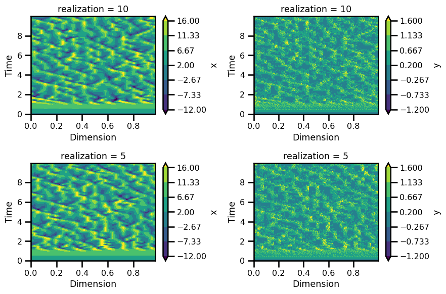
fig, ax = plt.subplots(nrows=2, ncols=2, figsize=(9, 6))

realization = 10
ds_sol.x.isel(realization=realization).plot.contourf(
    ax=ax[0, 0], cmap="viridis", vmax=16, vmin=-12
)
ax[0, 0].set_ylabel("Time")
ax[0, 0].set_xlabel("Dimension")


ds_sol.y.isel(realization=realization).plot.contourf(
    ax=ax[0, 1], cmap="viridis", vmax=1.6, vmin=-1.2
)
ax[0, 1].set_ylabel("Time")
ax[0, 1].set_xlabel("Dimension")

realization = 5
ds_sol.x.isel(realization=realization).plot.contourf(
    ax=ax[1, 0], cmap="viridis", vmax=16, vmin=-12
)
ax[1, 0].set_ylabel("Time")
ax[1, 0].set_xlabel("Dimension")


ds_sol.y.isel(realization=realization).plot.contourf(
    ax=ax[1, 1], cmap="viridis", vmax=1.6, vmin=-1.2
)
ax[1, 1].set_ylabel("Time")
ax[1, 1].set_xlabel("Dimension")

plt.tight_layout()
plt.show()