Lat-Lon Domains

J. Emmanuel JohnsonTakaya Uchida

import jax.numpy as jnp
import matplotlib.pyplot as plt
import numpy as np
import pandas as pd
import seaborn as sns
import xarray as xr
import jax
from jaxsw._src.domain.latlon import LatLonMeanDomain, LatLonDomain, lat_lon_deltas
from jaxsw._src.utils.coriolis import beta_plane, coriolis_param

sns.reset_defaults()
sns.set_context(context="talk", font_scale=0.7)
jax.config.update("jax_enable_x64", True)


%matplotlib inline
%load_ext autoreload
%autoreload 2

Latitude/Longitude Domains¶

Often we get data with spherical coordinates, i.e. latitude and longitude. This will be common when working with real data. So we need some way to convert the coordinates into a box-like domain.

Note: We could try to use a method that handles spherical coordinates out of the box. However, this is not available in this package (at the moment). See the xinvert package for details. (Might add this in at a later date)

Read input SSH¶

ds = xr.tutorial.open_dataset("ersstv5")
ds

lon = ds.lon.values
lat = ds.lat.values
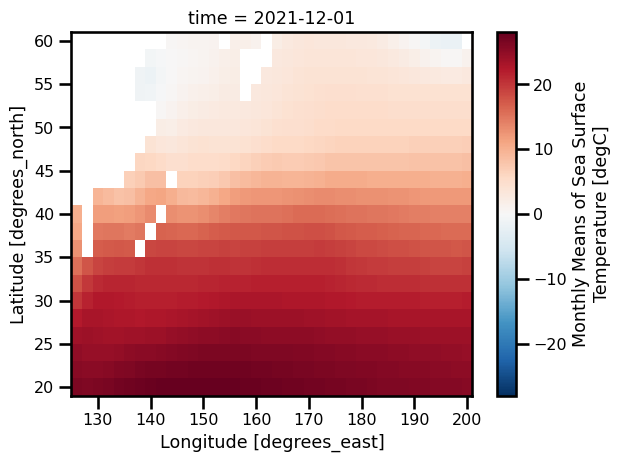
sst = ds.sst[0].values.T

subset_ds = ds.sel(lat=slice(60, 20), lon=slice(125, 200)).isel(time=-1)
subset_ds

fig, ax = plt.subplots()


# ds.sst.isel(time=-1).plot.pcolormesh(cmap="RdBu_r")
subset_ds.sst.plot.pcolormesh(cmap="RdBu_r")
plt.tight_layout()
plt.show()

Lat/Lon Domain¶

\text{lat(m)} =

(1)

d = \sqrt{(x_1 - x_2)^2 + (y_1 - y_2)^2}

(2)

# from metpy.calc import lat_lon_grid_deltas
# out = lat_lon_grid_deltas(lon, lat)

We look at the wiki page for the spherical Earth projected to a plane. Given some latitude, longitude pairs, $(\phi_1,\lambda_1), (\phi_2,\lambda_2)$ , we can calculate the distance between them:

\begin{aligned} \Delta\phi &= \phi_2 - \phi_1 \\ \Delta\lambda &= \lambda_2 - \lambda_1 \end{aligned}

(3)

We can also calculate the "mean" latitude

\phi_m = \frac{\phi_1 + \phi_2}{2}

(4)

Now we can calculate the distance between any set of points via the following formula:

d = R \sqrt{(\Delta \phi)^2 + (cos(\phi_m)\Delta\lambda)^2}

(5)

where $R$ is the radius of the Earth (6371200.0).

lon = subset_ds.lon.values
lat = subset_ds.lat.values

dx, dy = lat_lon_deltas(lon=lon, lat=lat)

print(dx.shape, dy.shape, lon.shape, lat.shape)

(38, 21) (38, 21) (38,) (21,)

f_0 = 2\Omega\sin(\text{lat}\frac{\pi}{180})

(6)

f = coriolis_param(lat)

f0 = jnp.mean(f)

print(f"Coriolis Param: {f0:.2e}")

Coriolis Param: 9.17e-05

This is very close to the parameter I've seen in simulations, i.e. $1e-5$

sst = jnp.asarray(subset_ds.sst[0].values.T)

Convenience Class¶

lon = subset_ds.lon.values
lat = subset_ds.lat.values

domain = LatLonMeanDomain(lat=lat, lon=lon)

assert domain.size == (lon.shape[0], lat.shape[0])

domain.size, domain.dx

((38, 21), (Array(170366.08, dtype=float32), Array(222396.9, dtype=float32)))

Many times, we're using a lot of approximate methods for the discretization and many of them require some uniform grid. There is a convenience method to simply take the mean of the dx.

domain.dx_mean

Array(196381.5, dtype=float32)