
Deep Markov Model#
Notes for the Deep Markov Model (DMM) algorithm.
Notes on Deep Markov Models (DMM) (aka Deep Kalman Filters (DKF))
State Space Model#
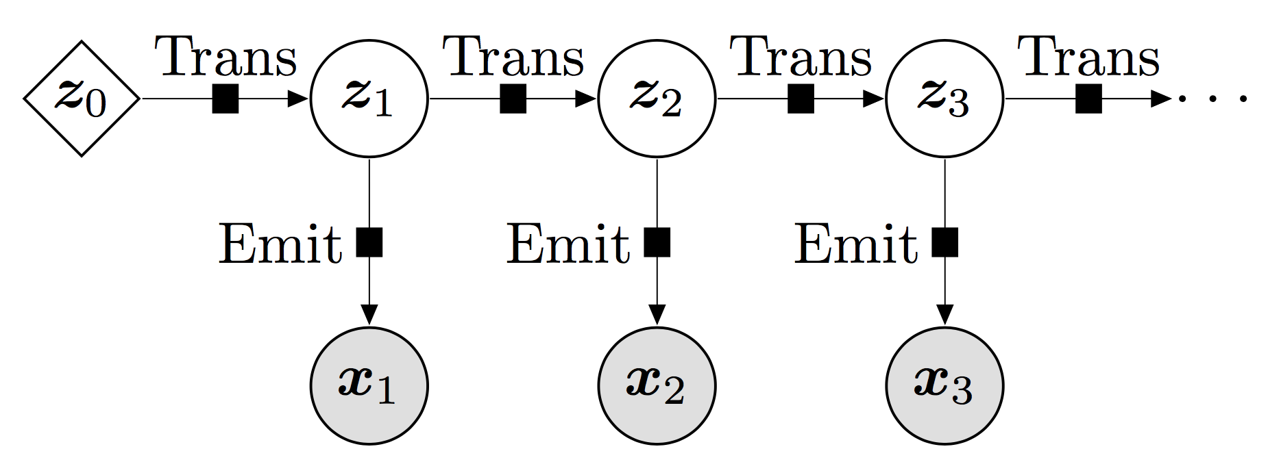
Fig. 9 This showcases the interaction between the hidden state and the observations wrt time. The most important property is the Markovian property which dictates that the future state only depends upon the current state and no other previous states obtained before. Source: pyro Deep Markov Model Tutorial.#
We are taking the same state-space model as before. However, this time, we do not restrict ourselves to linear functions. We allow for non-linear functions for the transition and emission functions.
We allow for a non-linear function, \(\boldsymbol f\), for the transition model between states.
We also put a non-linear function, \(\boldsymbol h\), for the emission model to describe the relationship between the state and the measurements. $\( \mathbf{x}_t = \boldsymbol{h}(\mathbf{z}_t; \boldsymbol{\theta}_e) + \boldsymbol{\epsilon}_t \)$(dmm_emission)
We are still going to assume that the output is Gaussian distributed (in the case of regression, otherwise this can be a Bernoulli distribution). We can write these distributions as follows:
where \(\theta_t\) is the parameterization for the transition model and \(\theta_e\) is the parameterization for the emission model. Notice how this assumes some non-linear transformation on the means of the Gaussian distributions however, we still want the output to be Gaussian.
If we are given all of the observations, \(\mathbf{x}_{1:T}\), we can write the joint distribution as:
If we wish to find the best function parameters based on the data, we can still calculate the marginal likelihood by integrating out the state, \(\mathbf{z}_{1:T}\):
Inference#
We can learn the parameters, \(\boldsymbol \theta\), of the prescribed model by minimizing the marginal log-likelihood. We can log transform the marginal likelihood function (eq (60)).
Loss Function#
Training#
We can estimate the gradients
Literature#
2D Convolutional Neural Markov Models for Spatiotemporal Sequence Forecasting - [Halim and Kawamoto, 2020]
Physics-guided Deep Markov Models for Learning Nonlinear Dynamical Systems with Uncertainty - [Liu et al., 2021]
Kalman Variational AutoEncoder - [Fraccaro et al., 2017] | Code
Normalizing Kalman Filter - [de Bézenac et al., 2020]
Dynamical VAEs - [Girin et al., 2021] | Code
Latent Linear Dynamics in Spatiotemporal Medical Data - Gunnarsson et al. (2021) arxiv
Model Components#
Transition Function#
where:
Functions#
Gate
gate = Sequential(
    Linear(latent_dim, hidden_dim),
    ReLU(),
    Linear(hidden_dim, latent_dim),
    Sigmoid(),
)
Proposed Mean
proposed_mean = Sequential(
    Linear(latent_dim, hidden_dim),
    ReLU(),
    Linear(hidden_dim, latent_dim)
)
Mean
z_to_mu = Linear(latent_dim, latent_dim)
LogVar
z_to_logvar = Linear(latent_dim, latent_dim)
Initialization
Here, we want to ensure that the output starts out as the identity function. This helps training so that we don’t start out with completely nonsensical results which can lead to crazy gradients.
z_to_mu.weight = eye(latent_dim)
z_to_mu.bias = eye(latent_dim)
Function
z_gate = gate(z_t_1)
z_prop_mean = proposed_mean(z_t_1)
# mean prediction
z_mu = (1 - z_gate) * z_to_mu(z_t_1) + z_gate * z_prop_mean
# log var predictions
z_logvar = z_to_logvar(nonlin_fn(z_prop_mean))
Emission Function#
where:
Tabular#
Gate
class Emission:
    def __init__(self, latent_dim, hidden_dim, input_dim) -> None:
        super().__init__()
        self.input_dim = input_dim
        self.z_to_mu = Sequential(
            Linear(latent_dim, hidden_dim),
            Linear(hidden_dim, hidden_dim),
            Linear(hidden_dim, input_dim)
        )
        self.hidden_to_hidden = Linear(hidden_dim)
Proposed Mean
proposed_mean = Sequential(
    Linear(latent_dim, hidden_dim),
    ReLU(),
    Linear(hidden_dim, latent_dim)
)
Mean
z_to_mu = Linear(latent_dim, latent_dim)
LogVar
z_to_logvar = Linear(latent_dim, latent_dim)
Initialization
Here, we want to ensure that the output starts out as the identity function. This helps training so that we don’t start out with completely nonsensical results which can lead to crazy gradients.
z_to_mu.weight = eye(latent_dim)
z_to_mu.bias = eye(latent_dim)
Function
z_gate = gate(z_t_1)
z_prop_mean = proposed_mean(z_t_1)
# mean prediction
z_mu = (1 - z_gate) * z_to_mu(z_t_1) + z_gate * z_prop_mean
# log var predictions
z_logvar = z_to_logvar(nonlin_fn(z_prop_mean))