
Markov Models#
In these notes, we walk through a model for modeling time-dependent data. By enforcing the Markov chain properties, we only have a variable at time, \(t\), depend on the variable at a previous time step, \(t-1\). This results in very efficient directed graph which leads to inference of order \(\mathcal{O}(T)\).
The main source of inspiration for this is the lecture from the Probabilistic ML course from Tubingen [Henning, 2020]. Some of the details we taken from the probabilistic machine learning textbook from Kevin Murphy [Murphy, 2012].
Motivation#
Consider a large dimensional dataset, e.g. a data cube. This will be of size:
But let’s assume that it is a spatio-temporal dataset. Then we can decompose the dimension, \(D\) into the following components.
High Dimensionality#
This is a very high dimensional dataset. For example, if we have a very long time series like \(1,000\) time steps, then we will have a massive \(D\)-dimensional vector for the input variable.
Time Dependencies#
These time dependences are very difficult to model. They are highly correlated, especially at very near, e.g. \(t-1\), \(t\), and \(t-1\).
Schematic#
This method seeks to decouple time by enforcing the Markov assumption.
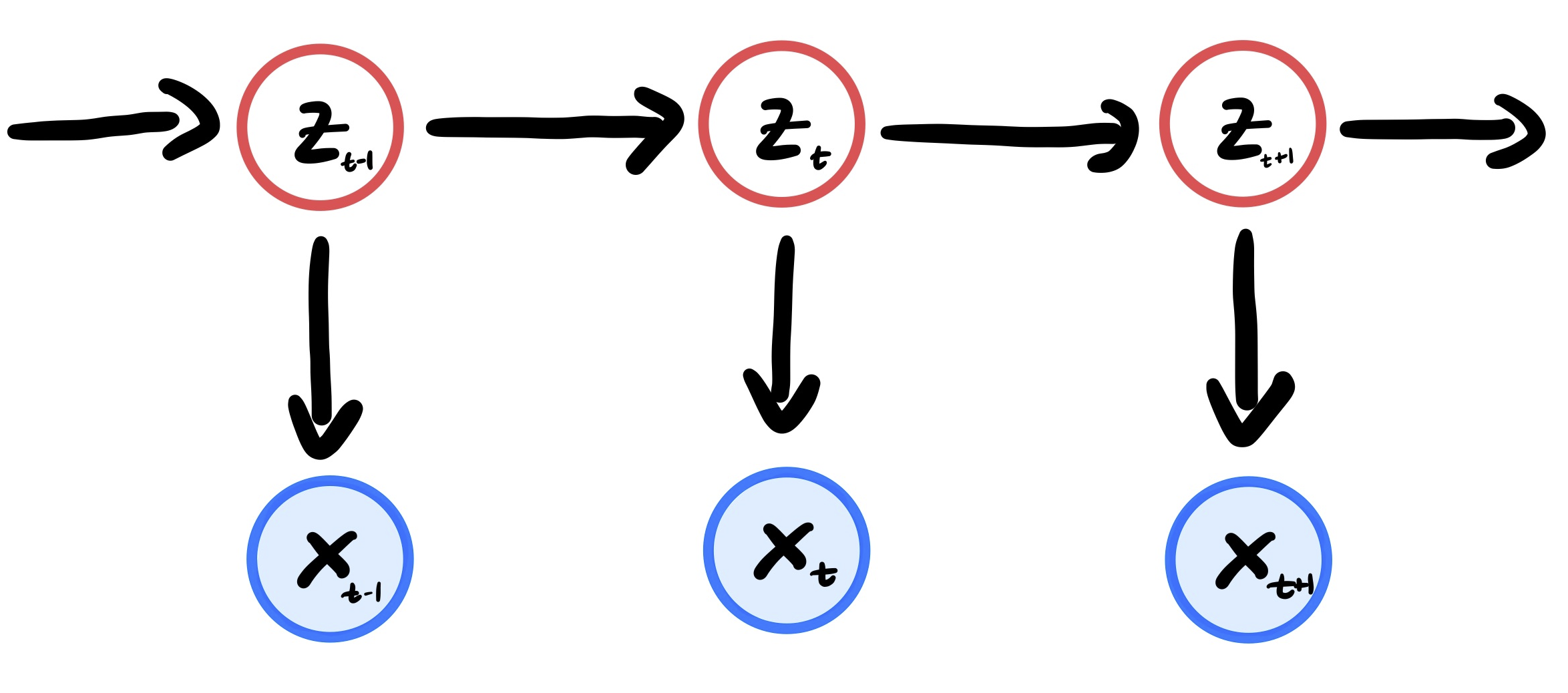
Fig. 8 A graphical model for the dependencies between the variables x and z. Notice how z only depends on the previous time step.#
The key is that by enforcing these Markovian assumptions, we have a directed graph structure that results in very efficient inference. This is all due to the Markov property due to the chain structure.
Markov Properties#
Property of States#
Given \(z_{t-1}\), \(z_t\) is independent of any other of the previous states, e.g. \(z_{t-2}, z_{t-3}, \ldots\).
This is enforcing some kind of local memory within our system. So even if we have the full system of observed variables, \(x_{1:T}\), and the posterior states, \(z_{1:T}\), we still only have the dependencies on the previous time step.
Bottom line: The past is independent of the future given the present.
Conditional Independence of Measurements#
We assume that the measurement, \(x_t\), given the current state, \(z_t\), is conditionally independent of the measurements and its histories.
So as you can see, the measurement at time, \(t\), is only dependent on the state, \(z\), at time \(t\) state irregardless of how many other time steps have been observed.
Joint Distribution#
While this may not be immediately useful, it is useful for certain other quantities of interest.
Using the Markov local memory and conditioning principal, we can decompose these conditionals wrt to the time, \(t\).
where we have all of the elements of the distribution.
Prior: \(p(z_0)\)
Transition Model: \(p(z_t|z_{t-1})\)
Observation Model: \(p(x_t|z_t)\)
Quantities of Interest#
Once we have the model structure, now we are interested in the specific quantities. All of them really boil down to quantities from inference.
TLDR#
Posterior - \(p(z_t|x_{1:t})\)
the probability of the state, \(z_t\) given the current and previous measurements, \(x_{1:t}\).
Predict Step - \(p(z_t|x_{1:t-1})=\int p(z_t|z_{t-1})p(z)\)
The current state, \(z_t\), given the past measurements, \(x_{1:t-1}\).
Measurement Step - \(p(z_t|x_t, x_{1:t-1}) \propto p(x_t|z_t)p(z_t|x_{1:t-1})\)
The current state, \(z_t\), given the present measurement \(x_t\) and past measurements, \(x_{1:t-1}\)
Marginal Likelihood - \(p(x_{1:T}) = \sum_{t}^T p(x_t|x_{1:t-1})\)
The likelihood of measurements, \(x_{1:T}\), given the state, \(z_{1:T}\).
Posterior Predictive: \(p(x_t|x_{1:t-1}) = \int p(x_t|z_t)p(z_t|z_{t-1})dz_t\)
The probability of the measurement, \(x_t\), given the previous measurements, \(x_{1:t-1}\).
Posterior Samples: \(z_{1:T} \sim p(z_t|x_{1:T})\)
Trajectories for states, \(z_{1:t}\), given the measurements, \(x_{1:T}\).
Sampling (Measurements): \(x_t \sim p(x_t|x_{1:t-1})\)
Trajectories for observations, \(x_{1:T}\), given the state space model, \(z_{1:T}\).
Filtering#
We are interested in computing the belief of our state, \(z_t\). This is given by
This equation is the posterior probability of \(z_t\) given the present measurement, \(x_t\), and all of the past measurements, \(x_{1:t-1}\). We can compute this using the Bayes method (eq (18)) in a sequential way.
Remark 2
The term filter comes from the idea that we reduce the noise of current time step, \(p(z_t|x_t)\), by taking into account the information within previous time steps, \(x_{1:t-1}\).
This is given by the predict-update equations.
Predict#
This quantity is given via the Chapman-Kolmogrov equation.
Term I: This is the posterior of \(z_t\) given all of the previous observations, \(x_{1:t-1}\).
Term II: the transition distribution between time steps.
Term III: the posterior distribution of the state, \(z_{t-1}\), given all of the observations, \(x_{1:t-1}\).
Note: term III is the posterior distribution but at a previous time step.
Filtering Algorithm#
The full form for filtering equation is given by an iterative process between the predict step and the update step.
1. Predict the next hidden state
First you get the posterior of the previous state, \(\mathbf{z}_{t-1}\), given all of the observations, \(\mathbf{x}_{1:t-1}\).
Second, you get the posterior of the current state, \(\mathbf{z}_t\), given all of the observations, \(p(\mathbf{x}_{1:t-1})\)
2. Predict the observation
First, you take the state, \(x_t\), given the previous measurements, \(y_t\).
Second you predict the current measurement, \(y_t\), given all previous measurements, \(y_{1:t-1}\).
3. Update the hidden state given the observation
First, you take the new observation, \(y_t\)
Then, you do an update step to get the current state, \(x_t\), given all previous measurements, \(y_{1:t}\).
Update#
Term I: The posterior distribution of state, \(z_t\), given the current and previous measurements, \(x_{1:t}\).
Term II: The observation model for the current measurement, \(x_t\), given the current state, \(z_t\).
Term III: The posterior distribution of the current state, \(z_t\), given all of the previous measurements, \(x_{1:t-1}\).
Term IV: The marginal distribution for the current measurement, \(x_t\).
Smoothing#
We compute the state, \(z_t\), given all of the measurements, \(x_{1:T}\) where \(1 < t < T\).
We condition on the past and the future to significantly reduce the uncertainty.
Remark 3
We can see parallels to our own lives. Take the quote “Hindsight is 22”. This implies that we can easily explain an action in our past once we have all of the information available. However, it’s harder to explain our present action given only the past information.
This use case is very common when we want to understand and learn from data. In a practical sense, many reanalysis datasets take this into account.
Term I: The current state, \(z_t\), given all of the past, current and future measurements, \(x_{1:T}\) (smoothing step)
Term II: The current state, \(z_t\), given all of the present and previous measurements, \(x_{1:t}\) (the predict step)
Term III: The “future” state, \(z_{t+1}\), given the previous state, \(z_t\) (transition prob)
Term IV: The “future” state, \(z_{t+1}\), given all of the measurements, \(x_{1:T}\).
Term V: The “future” state, \(z_{t+1}\), given all of the current and past measurements, \(x_{1:T}\).
Predictions#
We want to predict the future state, \(z_{T+\tau}\), given the past measurements, $x_{}.
where \(\tau > 0\). \(\tau\) is the horizon of our forecasting, i.e. it is how far ahead of \(T\) we are trying to predict. So we can expand this to write that we are interested in the future hidden states, \(z_{T+\tau}\), given all of the past measurements, \(x_{1:T}\).
We could also want to get predictions for what we observe
This is known as the posterior predictive density.
This is often the most common use case in applications, e.g. weather predictions and climate model projections. The nice thing is that we will have this as a by-product of our model.
Likelihood Estimation#
For learning, we need to calculate the most probable state-space that matches the given observations. This assumes that we have access to all of the measurements, \(x_{1:T}\).
Note: This is a non-probabilistic approach to maximizing the likelihood. However, this could be very useful for some applications. Smoothing would be better but we still need to find the best parameters.
Posterior Samples#
We are interested in generating possible states and state trajectories. In this case, we want the likelihood of a state trajectory, \(z_{1:T}\), given some measurements, \(x_{1:T}\). This is given by:
This is very informative because it can show us plausible interpretations of possible state spaces that could fit the measurements.
Remark 4
In terms of information, we can show the following relationship.
Marginal Likelihood#
This is the probability of the evidence, i.e., the marginal probability of the measurements. This may be useful as an evaluation of the density of given measurements. We could write this as the joint probabilty
We can decompose this using the conditional probability. This gives us
As shown by the above function, this is done by summing all of the hidden paths.
This can be useful if we want to use the learned model to classify sequences, perform clustering, or possibly anomaly detection.
Note: We can use the log version of this equation to deal with instabilities.
Complexity#
This is the biggest reason why one would do a Markov assumptions aside from the simplicity. Let \(D\) be the dimensionality of the state space, \(z\) and \(T\) be the number of time steps given by the measurements. We can give the computational complexity for each of the quantities listed above.
Filter-Predict
This is of order \(\mathcal{O}(D^2T)\)
If we assume sparsity in the methods, then we can reduce this to \(\mathcal{O}(DT)\).
We can reduce the complexity even further by assuming some special matrices within the functions to give us a complexity of \(\mathcal{O}(T D \log D)\).
If we do a parallel computation, we can even have a really low computational complexity of \(\mathcal{O}(D \log T)\).
Overall: the bottleneck of this method is not the computational speed, it’s the memory required to do all of the computations cheaply.
Viz#
Bars#
Regression#
Cons#
While we managed to reduce the dimensionality of our dataset, this might not be the optimal model to choose. We assume that \(z_t\) only depends on the previous time step, \(z_{t-t}\). But it could be the case that \(z_t\) could depend on previous time steps, e.g. \(p(z_t | z_{t-1}, z_{t-2}, z_{t-2}, \ldots)\). There is no reason to assume that
Multiscale Time Dependencies#
One way to overcome this is to assume
Long Term#
Philipp Henning. Probabilistic ml - lecture 12 - gauss-markov models. 2020. URL: https://youtu.be/FydcrDtZroU (visited on 2021-10-10).