Patching — sliding-window inference (intro)

Patching intro — sliding-window inference on a Sentinel-2 chip¶

This notebook walks through the canonical SpatialPatcher use case — splitting a raster into chips, running an operator per chip, and stitching the results back into a global field. The substrate is a real Sentinel-2 L2A scene over Lake Tahoe pulled from Microsoft Planetary Computer via the geostack.load_s2_chip helper.

We track array shapes after every operation so the data flow stays explicit. The same machinery powers the 05_patching_grids and 06_ml_patches_augment applied walkthroughs at the parent project level — read those for end-to-end NDVI / dNBR / classification flows.

import json

import matplotlib.pyplot as plt
import numpy as np
from geopatcher import (
    RasterField,
    SpatialBoxcar,
    SpatialCustom,
    SpatialGaussian,
    SpatialHann,
    SpatialOverlapAdd,
    SpatialPatcher,
    SpatialRectangular,
    SpatialRegularStride,
    SpatialTukey,
)
from geostack import LAKE_TAHOE_BBOX, load_s2_chip
from geotoolz import Lambda, Sequential
from geotoolz.patch_ops import (
    ApplyToChips,
    GridSampler,
    Stitch,
)

1. Load one real chip¶

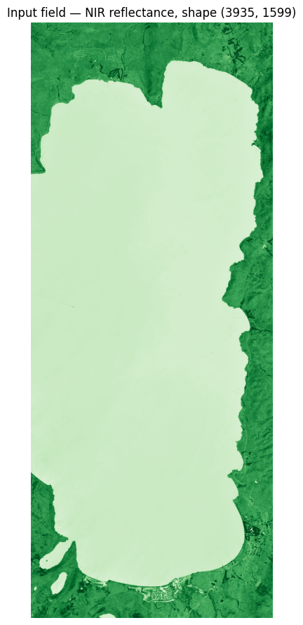
load_s2_chip does the STAC search + multi-band stacking + bilinear reprojection in one line. The returned GeoTensor is BGRN ((4, H, W) uint16) — for this intro we collapse to a single band (B08, NIR) so the patching arithmetic is easy to read; the applied walkthroughs use the full multi-band stack.

gt_bgrn = load_s2_chip(bbox=LAKE_TAHOE_BBOX)
print(f"S2 chip: shape={gt_bgrn.shape}  dtype={gt_bgrn.dtype}  crs={gt_bgrn.crs}")

nir_arr = np.asarray(gt_bgrn)[3].astype("float32") * 1e-4  # band-3 = NIR
gt = gt_bgrn.array_as_geotensor(nir_arr)  # (H, W) carrier
field = RasterField(gt)

fig, ax = plt.subplots(figsize=(7, 11))
ax.imshow(nir_arr, cmap="Greens", vmin=0, vmax=0.5)
ax.set_title(f"Input field — NIR reflectance, shape {nir_arr.shape}")
ax.axis("off")
plt.show()

S2 chip: shape=(4, 3935, 1599)  dtype=uint16  crs=EPSG:32610

2. The four-axis Patcher¶

256×256 SpatialRectangular patches, SpatialRegularStride of 256 (non-overlapping), SpatialBoxcar window (no taper), reconstruct via SpatialOverlapAdd.

patcher = SpatialPatcher(
    geometry=SpatialRectangular(size=(256, 256)),
    sampler=SpatialRegularStride(step=256),
    window=SpatialBoxcar(),
    aggregation=SpatialOverlapAdd(),
)

patches = list(patcher.split(field))
print(f"len(patches): {len(patches)}")
print(f"patches[0].data.shape: {np.asarray(patches[0].data).shape}")
print(f"patches[0].anchor: {patches[0].anchor}")
print(f"patches[0].indices: {patches[0].indices}")

len(patches): 90
patches[0].data.shape: (256, 256)
patches[0].anchor: (0, 0)
patches[0].indices: Window(col_off=0, row_off=0, width=256, height=256)

3. A window gallery¶

Before running an operator, let’s compare the five SpatialWindow classes. Each Window.weights(geometry) returns an array shaped like the patch — the multiplier OverlapAdd uses on the way in (per-cell) and the denominator on the way out (sum-of-weights).

windows_1d = {
    "Boxcar": SpatialBoxcar(),
    "Hann": SpatialHann(),
    "Tukey(α=0.3)": SpatialTukey(alpha=0.3),
    "Tukey(α=0.7)": SpatialTukey(alpha=0.7),
    "Gaussian(σ=0.3)": SpatialGaussian(sigma=0.3),
    "Gaussian(σ=0.6)": SpatialGaussian(sigma=0.6),
}
geom1d = SpatialRectangular(size=(1, 256))
fig, ax = plt.subplots(figsize=(8, 3.5))
for name, w in windows_1d.items():
    weights = w.weights(geom1d).reshape(-1)
    ax.plot(weights, label=name)
ax.set_title("1-D window profiles  —  weights.shape: (256,)")
ax.set_xlabel("patch index")
ax.set_ylabel("weight")
ax.legend(fontsize=8)
plt.show()

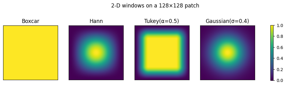
# 2-D view — same windows on a 128×128 patch
windows_2d = {
    "Boxcar": SpatialBoxcar(),
    "Hann": SpatialHann(),
    "Tukey(α=0.5)": SpatialTukey(alpha=0.5),
    "Gaussian(σ=0.4)": SpatialGaussian(sigma=0.4),
}
geom2d = SpatialRectangular(size=(128, 128))
fig, axes = plt.subplots(1, 4, figsize=(13, 3.3))
for ax, (name, w) in zip(axes, windows_2d.items(), strict=True):
    weights = w.weights(geom2d)
    print(f"{name:>16s}: weights.shape: {weights.shape}")
    im = ax.imshow(weights, vmin=0, vmax=1, cmap="viridis")
    ax.set_title(name)
    ax.set_xticks([])
    ax.set_yticks([])
fig.colorbar(im, ax=axes.ravel().tolist(), shrink=0.7)
plt.suptitle("2-D windows on a 128×128 patch")
plt.show()

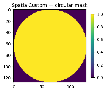
# `SpatialCustom` is the escape hatch — pass any callable
ring = SpatialCustom(
    fn=lambda g: (
        ((np.indices(g.size) - np.array(g.size)[:, None, None] / 2) ** 2).sum(axis=0)
        < (g.size[0] / 2) ** 2
    )
)
plt.figure(figsize=(4, 4))
plt.imshow(ring.weights(geom2d), cmap="viridis")
plt.title("SpatialCustom — circular mask")
plt.colorbar(shrink=0.7)
plt.show()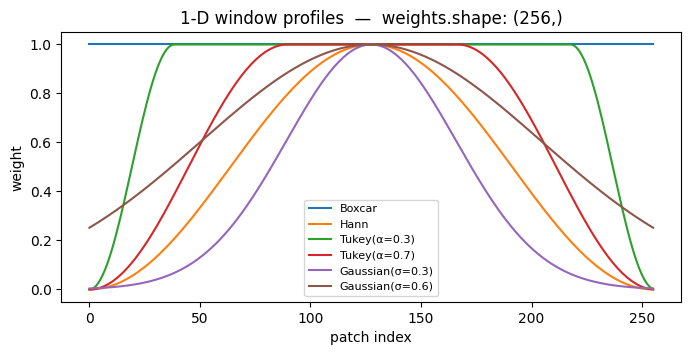

          Boxcar: weights.shape: (128, 128)
            Hann: weights.shape: (128, 128)
    Tukey(α=0.5): weights.shape: (128, 128)
 Gaussian(σ=0.4): weights.shape: (128, 128)

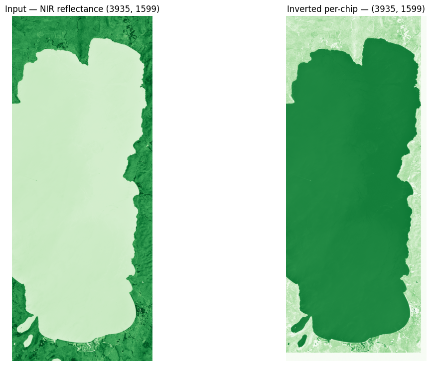
4. Per-chip operator: invert the gradient¶

A tiny Lambda operator that maps x → 0.5 - x. Inside each 256×256 chip it inverts the NIR-reflectance gradient — vegetation becomes dark, water becomes bright. Watching this run gives us a clean visual sanity check that the patches land in the right anchors and stitch back without seams.

invert = Lambda(lambda gt: 0.5 - np.asarray(gt), name="invert")

out_patches = ApplyToChips(invert)(patches)
print(f"len(out_patches): {len(out_patches)}")
print(f"out_patches[0].data.shape: {out_patches[0].data.shape}")

stitched = patcher.aggregation.merge(out_patches, field.reader)
print(f"stitched.shape: {stitched.shape}")

fig, axes = plt.subplots(1, 2, figsize=(13, 9))
axes[0].imshow(nir_arr, cmap="Greens", vmin=0, vmax=0.5)
axes[0].set_title(f"Input — NIR reflectance {nir_arr.shape}")
axes[0].axis("off")
axes[1].imshow(stitched, cmap="Greens", vmin=0, vmax=0.5)
axes[1].set_title(f"Inverted per-chip — {stitched.shape}")
axes[1].axis("off")
plt.show()

len(out_patches): 90
out_patches[0].data.shape: (256, 256)

stitched.shape: (3935, 1599)

5. Composition with `Sequential`¶

Same loop expressed as a three-operator linear pipeline using the gz.patch_ops wrappers. This is how the SpatialPatcher slots into the broader composition algebra.

pipe = Sequential(
    [
        GridSampler(patcher),
        ApplyToChips(invert),
        Stitch(SpatialOverlapAdd(), domain=field.reader),
    ]
)
result = pipe(field)
print(f"result.shape: {result.shape}")
np.testing.assert_allclose(np.asarray(result), stitched)
print("`Sequential` and the manual loop produce identical output ✓")

result.shape: (3935, 1599)

`Sequential` and the manual loop produce identical output ✓

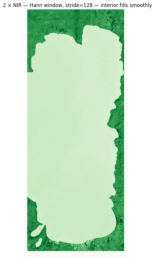
6. Hann window + overlap¶

Swap to a Hann window with stride < patch size. The OverlapAdd aggregation now normalises by the accumulated weights so the seams blend cleanly. Watch the seam between adjacent chips — it disappears entirely.

overlap_patcher = SpatialPatcher(
    geometry=SpatialRectangular(size=(256, 256)),
    sampler=SpatialRegularStride(step=128),  # 50 % overlap
    window=SpatialHann(),
    aggregation=SpatialOverlapAdd(),
)
double = Lambda(lambda gt: np.asarray(gt) * 2.0, name="double")

pipe2 = Sequential(
    [
        GridSampler(overlap_patcher),
        ApplyToChips(double),
        Stitch(SpatialOverlapAdd(), domain=field.reader),
    ]
)
out2 = np.asarray(pipe2(field))
print(f"out2.shape: {out2.shape}")

fig, ax = plt.subplots(figsize=(7, 11))
ax.imshow(out2, cmap="Greens", vmin=0, vmax=1.0)
ax.set_title("2 × NIR — Hann window, stride=128 — interior fills smoothly")
ax.axis("off")
plt.show()

out2.shape: (3935, 1599)

7. `get_config()` round-trip¶

Every axis (and the SpatialPatcher itself) returns a JSON-serialisable get_config() dict — the audit-trail artifact that lets you persist a pipeline as YAML or hash it for regulatory reproducibility.

print(json.dumps(patcher.get_config(), indent=2))

{
  "geometry": {
    "class": "SpatialRectangular",
    "config": {
      "size": [
        256,
        256
      ]
    }
  },
  "sampler": {
    "class": "SpatialRegularStride",
    "config": {
      "step": 256
    }
  },
  "window": {
    "class": "SpatialBoxcar",
    "config": {}
  },
  "aggregation": {
    "class": "SpatialOverlapAdd",
    "config": {
      "streaming": false,
      "target_path": null,
      "chunks": null,
      "normalize_by_window": true
    }
  }
}

Where next¶

02_geometries — the five geometry classes (Rectangular, SphericalCap, KNNGraph, RadiusGraph, PolygonIntersection) on real heterogeneous substrates.
03_sampling — the sampler gallery (RegularStride, JitteredStride, Random, PoissonDisk, Explicit).
06_streaming — same patcher pattern but at full S2 tile scale (~10980² px) using a zarr-backed SpatialOverlapAdd.
../05_patching_grids — the applied walkthrough version: NDVI over Lake Tahoe with a real per-chip operator stack.