
Input Uncertainty in GPs#
Notebook to reproduce the plots.
In real-world applications, we often need to consider uncertain inputs in our machine learning models. Every instrument we use to collect data will have some level of uncertainty and this is often explicitly available in certain datasets like observational products (cite: HSTAFR, FAPAR, etc) and satellite datasets (cite: IASI). Alternatively, we could have inputs from from other models like a trained regressor which would also have uncertainty. Not including this information into our datasets can have adverse effects on our predictions and uncertainty as we are not actually propagating error through our model. So we should definitely take this information into consideration when choosing the appropriate model. In this first section, we will set up the problem and cover some of the methods literature found in the literature.
History#
In traditional statistical models, accounting for uncertain inputs is known as error-in-variables (cite: Kendall & Stuart, 1958) a form of linear regression. There were a few competing ways in the literature of the relationship of how the inputs could be described: 1) we observe a noise corrupted version of the inputs, 2) we observe the actual inputs and assume the noise is independent. With either method, it’s difficult to estimate the true inputs and model parameters. A deterministic approach was to use moment reconstruction (cite: Freedman et al 2004, Freedman et al., 2008) which is an idea similar to regression calibration (cite: Hardin et al, 2003). More Bayesian approaches were to (cite: Snoussi et al, 2002; Spiegelman et al., 2011) used an modified expectation maximization scheme and treated the inputs as hidden variables and (cite: Dellaportas and Stephens, 1995) used Gibbs sampling to perform inference.
In other fields, there have been some attention in fields such as stochastic simulation (cite: Lam, 2016) and GP optimization schemes (cite: Wang et al 2019-GPOpt)
Predictions#
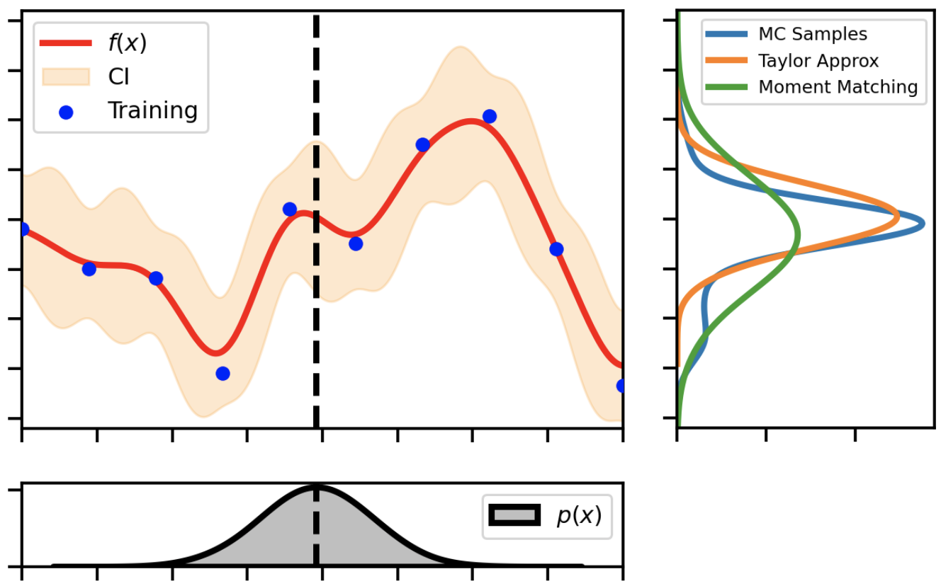
Fig. 2 A demonstration showing how an uncertain input propagates through a non-linear GP function.#
In Gaussian processes, the original formulation dictates that we assume there is some noise in the observations, \(y\) and that we observe the real inputs \(\mathbf{x}\). So we’ll see that this it is not trivial to modify this formulation to account for uncertain inputs. Let’s assume that we have a data set \(\mathcal{D}=\{\mathbf{X}, \boldsymbol{y} \}\). In this case we assume the following relationship between our inputs, \(\mathbf{x}\), and outputs, \(y\):
Let’s also assume that we have a standard GP model optimized and fitted to this data set. We’re not assuming noisy inputs during the training phase so we will use the standard log-likelihood maximization procedure. However, during the testing phase, we will assume that our inputs are noisy. For simplicity, we can assume our test data set is normally distributed with a mean \(\mu_\mathbf{x}\) and variance \(\Sigma_\mathbf{x}\). So we will have:
or equivalently we can reparameterize it like so:
If we consider the predictive distribution given by \(p(f_*|\mathbf{x}_*, \mathcal{D})\), we need to marginalize out the input distribution. So the full integral appears as follows.
If we use the GP formulation, we have a closed-form deterministic predictive distribution for \(p(f_*|\mathbf{x}_*,\mathcal{D})\). Plugging this into the above equation gives us:
So this integral is intractable because if we consider the terms within the GP predictive mean and predictive variance, we will need to calculate the integral of an inverse kernel function, \(\mathbf{K}_\mathcal{GP}^{-1}\). Below we outline some of the most popular methods found in the literature.
Monte Carlo#
The most exact solution would be to use Monte-Carlo simulations. We draw \(T\) samples from the distribution of our \(\mathbf{x}\sim \mathcal{N}(\mathbf{x}_*|\mu_\mathbf{x},\Sigma_\mathbf{x})\) and propagate this through the predictive mean and standard deviation of the Gaussian process .
to obtain our samples. This will be exact as the number of MC samples, \(T\) grows. In addition, one could use any distribution they want to represent the inputs \(\mathbf{x}\) like the T-Student for more noisy scenarios. The downside is that this method can be very expensive as we will have propagate our inputs through the predictive mean function \(T\) times. This is especially true for the exact GP but possibly can be mitigated by more sparse approximations (cite: SVGP, Unified)or better sampling schemes (cite: pathwise, GPyTorch-CQ). This method hasn’t been demonstrated in real world examples, only in toy examples in a PhD thesis of (cite: Girard). There has been many developments in the literature with regards to MC methods especially in relation to GPs including Gibbs sampling (cite: ), Elliptical slice sampling (cite: ), and NUTS (cite: ). MC methods have gotten more efficient over the years and so this method has the potential to be critical in applications with high uncertainty and a more thorough investigation of the parameters is needed especially with small-medium data problems.
Gaussian Approximation#
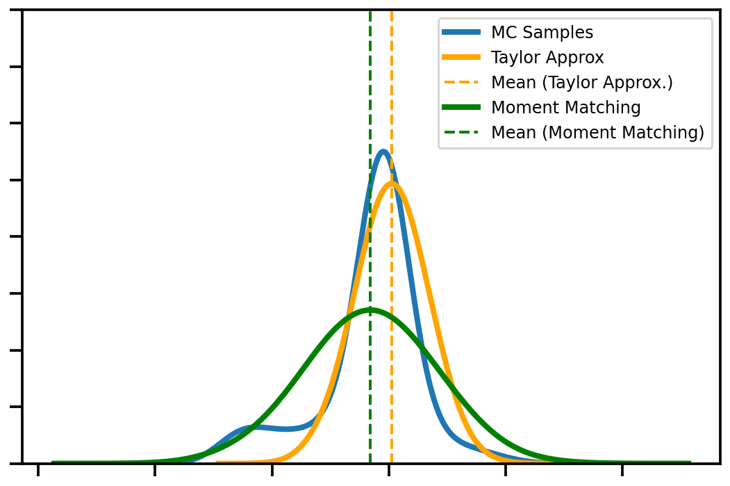
Fig. 3 A closer look at the shape of the posteriors for each of the uncertain operations (Taylor, Moment Matching) versus the golden standard Monte Carlo sampling.#
The integral of the GP predictive distribution is intractable as mentioned before so we need a way to approximate this distribution. In this family of methods, we approximate the predictive distribution as a Gaussian with the first and second moments. We can compute the moments of the predictive mean and variance equations by using the law of iterative expectations (cite: Fubinis theorem).
So our final sets of equations involve expectations over varying degrees of the predictive mean and variance equations for the GP algorithm. There are two competing methods in the literature for computing the expectations and variances of the predictive mean and variance: linearization and moment-matching. Linearization entails approximating the expectation with a Taylor expansion and moment-matching entails computing the moments exactly and then approximating the remaining integrals with quadrature methods like Gauss-Hermite or Unscented transformations. The Taylor transformation is easier to compute but less exact whereas the moment matching method is more exact but more expensive to compute. In paper 2, we chose the linearization approach but we will outline below the details of both approaches as well as some other approaches.
Taylor Expansion#
This is the simplest approach that is found in many of the earlier uncertain input GP literature. In this framework, we approximate the expected predictive mean and variance via a first and second order Taylor. Using this expansion, it is easier to compute the first and second moments (mean and variance) of the predictive distribution. This is a relatively fast and approximate method incorporate information into the predictive variance without needing to retrain the GP model. The equations are summarized below:
As shown, we still include the original predictive mean and variance terms (see appendix for the full derivation). In the end, this approximation augments the predictive mean and variance equations with terms that incorporate the first derivative of the predictive mean (1st order) and the second derivative of the predictive mean and variance (2nd order). This was originally proposed by (cite: Girard, Girard + Murray) as they were able to augment the gaussian process predictive mean and variance with the derivative of the predictive mean and the trace of the predictive variance. Subsequently, we saw other approaches (cite: Oakley and O’Hagan, 2002; Quinonero-Candela et al., 2003; Oakley, 1999,2004) implement the same strategy with great success on dynamical problems.
(cite: McHutchon) modeled this during the training regime as well by incorporating the linearization term into the GP likelihood. The results were promising and the confidence intervals were better. However, due to including the derivative of the kernel in the formulation, this resulted in a cyclic optimization scheme where one would need to optimize, find the derivative, repeat until convergence which is an expensive operation. In general in today’s literature, this is not the dominant method used although (cite: Deisenroth) referenced this method as a good alternative when one needs an easy and scalable approximation and it was revisited as an alternative in GP classification (cite: Lobato). Please see (cite: Girard (Tech Report), Bijl) for the full derivation.
Moment Matching#
This is one of the most commonly used methods to date for dealing with uncertain predictions in GPs. It works by computing the first and second moments of the new predictive distribution and then applying quadrature methods to solve all of the remaining integrals. So explicitly, we need to take expectations (integrals) of the GP predictive mean and variance w.r.t. our distribution for \(\mathbf{x}_*\).
After some manipulation, this results in the follow equations for the predictive mean and variance (cite).
where we have \(\Psi_i\) quantities called kernel expectations denoted by:
Notice how we have expectations where we need to use quadrature methods to calculate these quantities. So compared to the linearization approach, this will give us a more exact solution and better representation than the Taylor approximation especially for more complex functions. This method was used in (cite: Girdard,Candela) for dynamical time series problems and later it become more popular in applications such as the PILCO problem where (cite: Deisenroth) used the same formulation. Later, this method was seen in more recent GP developments like the Bayesian GPLVM (cite: Titsias) and the original Deep GP (cite: Damianou) where they use the variational approach (more below). See (cite: Deisenroth, Dutodoir, Bijl) for the full derivation of the above equations or appendix for a more succinct version.
This is often the preferred method for many applications with uncertain predictions. One advantage is the geometric meaning as it is akin to approximating the forward KL-Divergence between a prior \(p\) and an approximate variational distribution \(q\), i.e. \(\text{KLD}[p||q]\). The moment matching distribution is similar to the approximate variation distribution \(q\) and the uncertain input data is similar to the prior term \(p\) (ref: figure)(cite: Deisenroth thesis, 2010). The forward KL is a conservative estimate to ensure all regions of \(p(x)>0\) is covered by \(q(x)\). This is very similar to the approach taken by the \(\alpha\)-divergence and expectation propagation when \(\alpha=1\) (cite: ). However practically, this is an expensive measure to calculate due to the kernel expectations. It is only exact to specific kernel functions that have been derived like the linear, RBF (cite: Girard, McHutchon, Damianou) and spectral kernel (cite: Vincent). In all other cases, the integrals need to be approximated via quadrature methods. Gauss-Hermite is the most popular method found in standard GP toolboxes (cite: GPy, GPFlow, GPyTorch) but there have been explorations to use unscented transform (cite: ) which are more scalable and are exact enough in lower dimensional settings.
Toy Example#
Now, we want to demonstrate how each of these methods perform and how well they improve the confidence intervals of the data. In this toy example, we will look at how each of the methods compare. More specifically, we will look at the confidence intervals and see if they sufficiently capture the outliers. We have a standard GP and we see that the confidence intervals do not sufficiently encapsulate the noisy inputs.
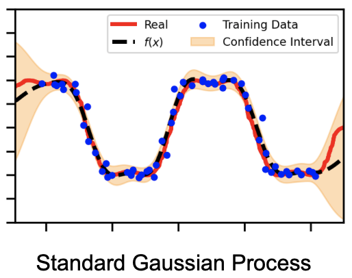
Fig. 4 A closer look at the shape of the posteriors for each of the uncertain operations (Taylor, Moment Matching) versus the golden standard Monte Carlo sampling.#
Whereas we see the other methods do a better job. The MC method is the golden standard and the other methods are more Gaussian approximations. Although they are approximations, they still do a better job at capturing the input noise.
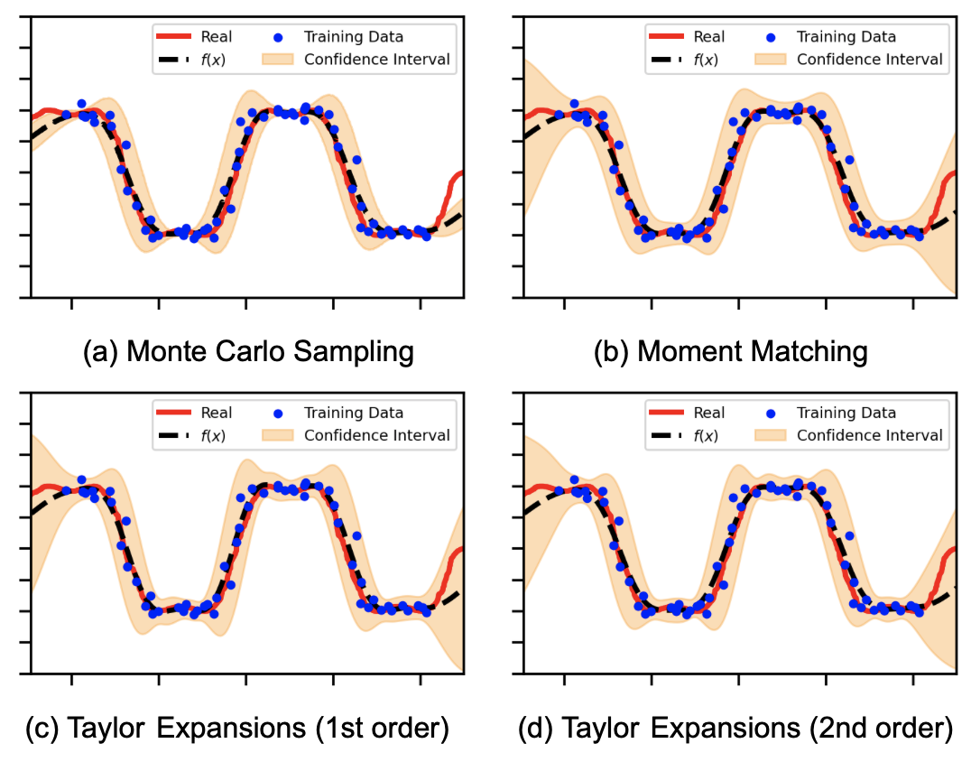
Fig. 5 A closer look at the shape of the posteriors for each of the uncertain operations (Taylor, Moment Matching) versus the golden standard Monte Carlo sampling.#
Next Steps#
In the above methods, they assume that a GP regression algorithm has already been trained on a dataset \(\mathcal{D}\). They are advantageous because they are relatively simple and we can use the exact GP formulation for our training procedures and However, in the case where we have the whole data set with the noisy inputs \(\mathbf{x}\), and \(y\), this is not a good assumption and ideally we would want to take the whole dataset into account. For most of the intended applications above, they were focused on dynamical systems with time series so propagating error was very important.
Kernel Functions#
Another frame of thinking involved modifying the kernel function to allow one to include error in. This is advantageous as it allows one to incorporate the uncertainty into the training of the GP method in addition to the testing without having to use approximate posterior methods (see latent variables). In one method (cite: Dallaire), the motivation was to modify the length scale of the RBF kernel to account for the covariance within the inputs. The limitations of this method is that it assumes a constant covariance for each of the inputs which isn’t flexible and also (cite: McHutchson) found that the length scales describing the RBF kernel function collapses to the scale of the covariance. Surprisingly, this approach hasn’t been explored more seeing how a common limitation of Gaussian process methods is the expressiveness of the kernel function (cite: Bonilla-AGP) and so creating a kernel to incorporate the error in the inputs would be a clever way to mitigate this issue. For example, (cite: Moreno-KLDKernel) created a specialized kernel based off of the KL-Divergence which works for Gaussian noise inputs. Even though this isn’t a valid kernel (cite: blog), the results showed improvement. Deep kernel learning (cite: Wilson) is an example of a fully parameterized kernel functions via neural networks which would allow uses to use methods like the noise constrastive prior (cite: NCP) to deal with noisy inputs.
Heteroscedastic Likelihoods#
In this field of literature, the problem is transformed to finding a parameterized function. The challenge is that this cannot be applied to the exact GP model because it won’t be an explicit Gaussian likelihood which is non-conjugate and thus we would require approximate inference methods like variational inference or expectation propagation or sample-based schemes like Monte Carlo schemes.
Literature
Kersting et al 2007
Golbery et al 1998
Lazaro-Gredilla and Titsias, 2011
Latent Variables#
Another approach to incorporate noise into the inputs is to assume that the inputs are a latent variables. We presume to observe the noisy versions of the real variable \(\mathbf{}\). We would specify a prior distribution over
From a practical perspective, there are many options for the practioner to configure the trade-off between the prior configuration and the variational configuration. For example, we could be very loose with our assumptions by intializing the prior with the mean of the noisy inputs and then let both the prior and the variational distribution be a free parameters. Or we could be very strict with our assumptions and set the prior and variational distributions to be our
Connection to MM Methods#
We can make the connection that
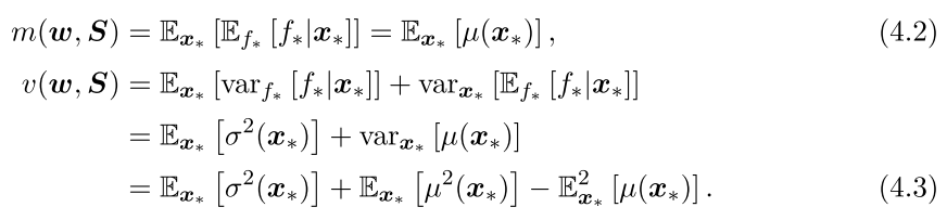
Fig. 6 Efficient Reinforcement Learning using Gaussian Processes#
Thoughts#
So after all of this literature, what is the next step for the community? I have a few suggestions based on what I’ve seen:
Apply these algorithms to different problems (other than dynamical systems)
It’s clear to me that there are a LOT of different algorithms. But in almost every study above, I don’t see many applications outside of dynamical systems. I would love to see other people outside (or within) community use these algorithms on different problems. Like Neil Lawrence said in a recent MLSS talk; “we need to stop jacking around with GPs and actually apply them” (paraphrased). There are many little goodies to be had from all of these methods; like the linearized GP predictive variance estimate for better variance estimates is something you get almost for free. So why not use it?
Improve the Kernel Expectation Calculations
So how we calculate kernel expectations is costly. A typical sparse GP has a cost of \(O(NM^2)\). But when we do the calculation of kernel expectations, that order goes back up to \(O (DNM^2)\) . It’s not bad considering but it is still now an order of magnitude larger for high dimensional datasets. This is going backwards in terms of efficiency. Also, many implementations attempt to do this in parallel for speed but then the cost of memory becomes prohibitive (especially on GPUs). There are some other good approximation schemes we might be able to use such as advanced Bayesian Quadrature techniques and the many moment transformation techniques that are present in the Kalman Filter literature. I’m sure there are tricks of the trade to be had there.
Think about the problem differently
An interesting way to approach the method is to perhaps use the idea of covariates. Instead of the noise being additive, perhaps it’s another combination where we have to model it separately. That’s what Salimbeni did for his latest Deep GP and it’s a very interesting way to look at it. It works well too!
Think about pragmatic solutions
Some of these algorithms are super complicated. It makes it less desireable to actually try them because it’s so easy to get lost in the mathematics of it all. I like pragmatic solutions. For example, using Drop-Out, Ensembles and Noise Constrastive Priors are easy and pragmatic ways of adding reliable uncertainty estimates in Bayesian Neural Networks. I would like some more pragmatic solutions for some of these methods that have been listed above. Another Shameless Plug: the method I used is very easy to get better predictive variances almost for free.
Figure Out how to extend it to Deep GPs
So the original Deep GP is just a stack of BGPLVMs and more recent GPs have regressed back to stacking SVGPs. I would like to know if there is a way to improve the BGPLVM in such a way that we can stack them again and then constrain the solutions with our known prior distributions.
Posterior Approximations#
Post Training#
Monte Carlo Sampling#
Moment-Matching#
Gauss-Hermite
Unscented Transforms
During-Training#
Distribution Kernels#
Latent Variables#
Latent Co-Variate Models#
Neural Networks#
Deep Gaussian Processes#
Naturally deal with uncertain inputs
More expressive
Not clear about error propagation
Contribution & Impact#
Conclusions#
Uncertain Predictions#
Monte Carlo Sampling
Moment Matching
GPs w/ Training Data#
Stochastic Variational GPs
Bayesian Latent Variable Model
Deep Gaussian Processes
Normalizing Flows (Hybrid Models)