Interpolation Problem

Interpolation Problem#

../../../_images/oi_grid.png — Fig. 7 Here is my figure caption! Source: tweet#

Planned TOC#

Background#

Optimal Interpolation#

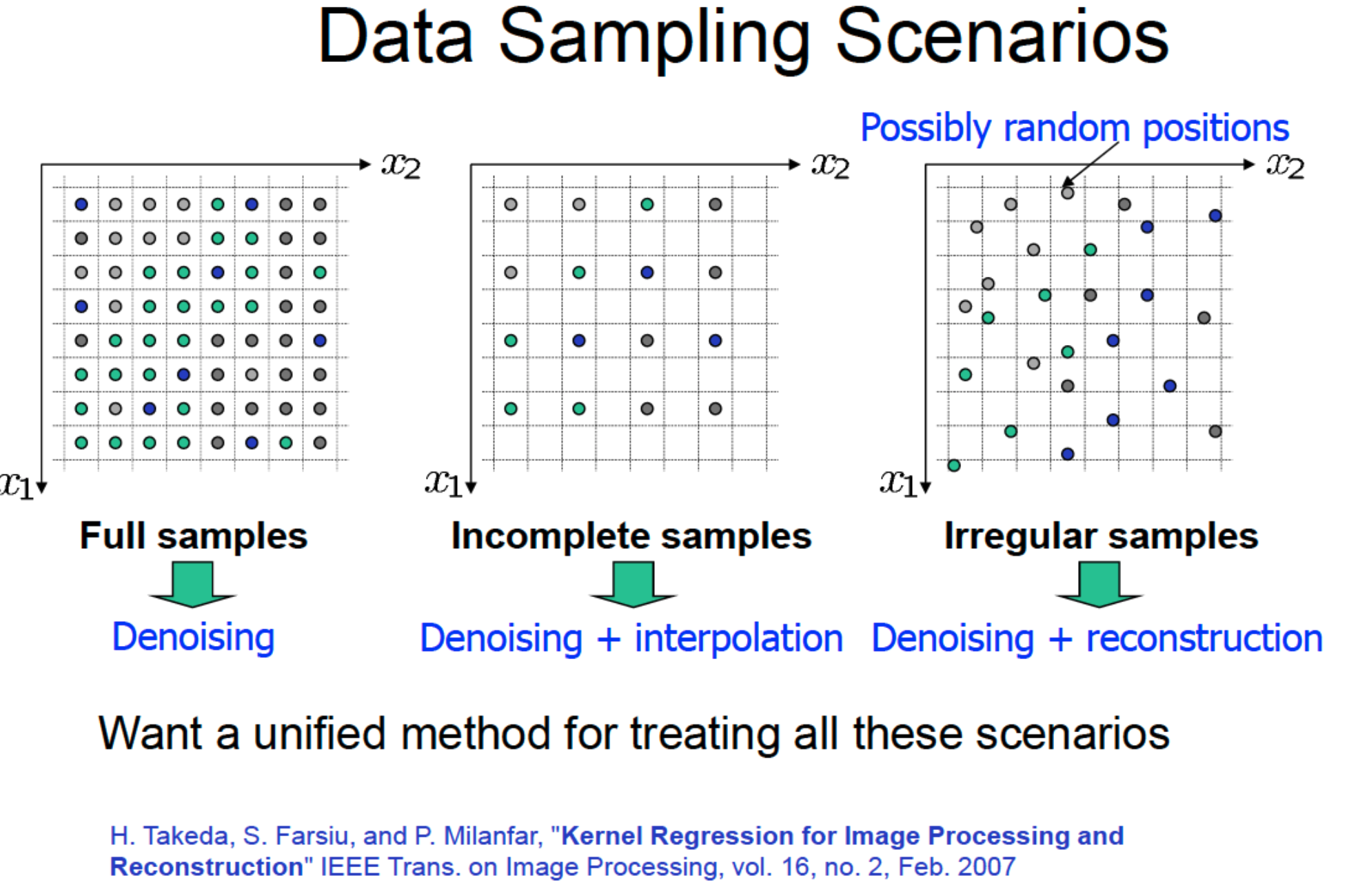
Optimal Interpolation (OI) seems to be the golden standard for gap-filling SSH fields with missing data. Something that is very prevalent for Satellite sensors. However, the standard OI method

\[\begin{split} \begin{aligned} \tilde{\boldsymbol{\mu}}_{\mathbf{x}_{t}} &= \mathbf{x}_t + \mathbf{K}(\mathbf{y}_t - \mathbf{H}\mathbf{x}_t) \\ \tilde{\boldsymbol{\Sigma}}_{\mathbf{x}_{t}} &= (\mathbf{I} - \mathbf{KH})\boldsymbol{\Sigma}_\mathbf{x} \\ \mathbf{K} &= \mathbf{P} \mathbf{H}\left(\mathbf{H} \mathbf{P} \mathbf{H}^\top + \mathbf{R} \right)^{-1} \\ \end{aligned} \end{split}\]

The \(\mathbf{K}\) is known as the Kalman gain. The optimal \(\mathbf{K}\) is given by:

\[ \mathbf{K} = \boldsymbol{\Sigma}_{\mathbf{xy}} \boldsymbol{\Sigma}_{\mathbf{yy}}^{-1} \]

where \(\boldsymbol{\Sigma}_{\mathbf{yy}}\) is the covariance between the observations and \(\boldsymbol{\Sigma}_{\mathbf{xy}}\) is the cross-covariance between the state and the observations.

Notice how this assumes that interpolation can be done via a linear operator, \(\mathbf{H}\). The Kalman gain, \(\mathbf{K}\), represents the best interpolation via this linear problem. However, this is often insufficient in many scenarios where the data does not exhibit linear dynamics.

Kernel Methods#

This is similar to the kernel ridge regression (KRR) and Gaussian process (GP) formulation.

\[\begin{split} \begin{aligned} \boldsymbol{\mu}(\mathbf{x}^*) &= \boldsymbol{k}_{\mathbf{x}}(\mathbf{x}^*) \boldsymbol{\alpha} \\ \boldsymbol{\Sigma}(\mathbf{x}^*, \mathbf{x'}^*) &= \boldsymbol{k}(\mathbf{x}^*, \mathbf{x}^*) - \boldsymbol{k}_{\mathbf{x}}(\mathbf{x}^*)(\mathbf{K_{XX}} + \sigma^2\mathbf{I})^{-1} \boldsymbol{k}_{\mathbf{x}}(\mathbf{x}^*)^\top \\ \boldsymbol{\alpha} &= (\mathbf{K_{XX}} + \sigma^2\mathbf{I})^{-1}\mathbf{y} \end{aligned} \end{split}\]

Notice how \(\boldsymbol{\alpha} \in \mathbb{R}^{N}\) is simply a weight that gets multiplied by the cross-covariance, \(\boldsymbol{k}(\mathbf{x}^*)\) for the new observations. The advantage of this is that it allows for mean predictions and variance predictions. The big bottleneck of this method is that we have to invert the \(\mathbf{K_{XX}}^{-1}\) which is of order, \(\mathcal{O}(N^3)\). Often times we don’t need so many observations to be able to efficient capture the essence of the data. For example, we can approximate this method by assuming we can decompose this kernel matrix into a lower dimensional matrix, \(\mathbf{L} \in \mathbb{R}^{D \times d}\) s.t.

\[ \mathbf{K} = \mathbf{LL}^\top \]

Methods like this are data independent like random Fourier features or random projection methods. Another methods assume we can decompose the matrix into a low-rank matrix like so:

\[ \mathbf{K} = \mathbf{K_r}\mathbf{K_{rr}}^{-1}\mathbf{K_r} \]

This is a data-dependent method, eg. the Nystrom approximation. With a big of math magic, it is relatively straightforward to modify the above predictive mean and variance equations based on sparse matrix approximations listed above. This results in scalable of order \(\mathcal{O}(NM^2)\) which can drastically speed up learning as well as predictions.

Kriging#

The application of kernel methods (in particular GPs) has been widely used in the geostatistics literature.

PyKrige

Kernel Functions#

This is the most important aspect of the . In the code I inherited, I saw that they use the Gaussian kernel (aka RBF, Squared Exponential) which gives us smooth solutions. This is the most widely used kernel function in the literature because it is a universal approximator and serves as a good baseline because it exhibits desireable properties, e.g. smoothness, differentiable, etc. However, in the case of ocean data, smoothness might be detrimental to our application if we don’t expect smooth solutions.

Another powerful aspect is the combination of kernel functions. For example, the following kernel operations are valid kernels:

\[\begin{split} \begin{aligned} K &= K + K \\ K &= K * K \\ \end{aligned} \end{split}\]

This gives rise to potentially more expressive kernel functions as combinations. For example, in the classic Moana Loana example, we find that thinking about the potential dynamics at play help us to design good kernel functions that can describe the dynamics of the data. In other applications, kernel functions that exhibit stronger periodicity might be better suited to the problem, e.g. spectral mixture kernel.

In extra step is to do deep kernel learning (DKL) whereby we use a neural network as a flexible, non-linear feature extractor before inputing this into a kernel function itself (example). We lose the interpretation aspect because we offload all non-linearities into the neural network, however this allows for us to capture dynamics that cannot be approximated via clever combinations of kernel functions.

Uncertainties#

These is quite an easy jump to an interpolation method that is able to give good predictive uncertainties. GPs remain the gold standard for predictive uncertainties that actually make sense. While there are many probabilistic and Bayesian neural networks in the literature, the predictive variances they give are often nonsensical and can lead to incorrect decisions down the line.

Furthermore, there are many efficient methods to generate samples within the KRR and the GP settings. This can be useful in a setting where we want to quickly emulate samples just based on observations; something that the 4DVarNet can use to better characterize the uncertainty for missing observations.

Software#

We can use the scikit-learn library as the preliminary exploration library. They have an implementation of KRR and a simple GP that can be used as a prototype for the initial exploration. They also have many kernel functions available for us to explore. We can also utilize some of the standard ML practices for learning the parameters, e.g. randomized or brute-force grid searches.

Demonstration: I think this can offer people a learning experience for utilizing kernel methods from a machine learning perspective. I think we can focus on some key toy problems to try and illustrate the power. I personally have developed a lightweight JAX library, jaxkern, library for implementing some basic kernel methods. And I am also a regular contributor to the GPJax for the more probabilistic perspective.

Scalability: For the scalable methods, scikit-learn offers a few solutions to kernel approximation including the random Fourier features methods, the Nystroem approximation and TensorSketch methods. However, if we hope to incorporate this into a differentiable framework, we need to use other backends such as PyTorch. However, more heavy duty libraries such as KeOPs (written in Numpy and PyTorch) has shown to scale to billions of observations, e.g. in KRR and GPyTorch.

Hypothesis#

I believe there is a lot to be explored regarding the family of kernel methods. For example, we have the freedom to choose the kernel function, \(\boldsymbol{k}\), which can encode certain properties that we expect the data to exhibit. Furthermore, we can operate these parameters based upon the data. In addition, one can solve for the best parameters, \(\boldsymbol{\theta}\), once and then simply apply this on new datasets. The kernel method literature vast and . Lastly, the use of kernel methods in oceanography has not been studied in great detail and this provides us with an opportunity to lead the community in this perspective.

Connections to Other Methods#

DUACS

There are notes from the original paper and the original formulation. They mention how the BLUE estimator is limited if there is no prior knowledge and that one can estimate the covariances directly from the data. However, the connection has not been explored in great detail. For example, nothing is said about the chosen kernel functions nor the training strategies.

4DVarNet

This algorithm requires a good initial condition for solving the minimization problem:

\[ \mathbf{x}^* = \argmin_{\mathbf{x}} \boldsymbol{U}(\mathbf{x}_{\text{init}}, \mathbf{y}_{\text{obs}}, \boldsymbol{\theta}) \]

There are quite a few cases where a bad initial condition will result in local minimum or poor solutions. A great initialization can alleviate some of the difficulties of the 4DVarNet.

Kalman Filters

The Gaussian process method with a linear kernel function, \(\boldsymbol{k}\), is equivalent to the Kalman filter. They produce the exact same solution, however, the KF solves the problem sequentially whereas the GP solves the problem with all of the data. In the above proposal, we go beyond linear kernels which gives us extra flexibility. However, later, scalability might still be an issue as well as longer time scales. In this case, Markovian GPs have found a lot of recent success in sequential data. They are approximate continuous counterparts to the Kalman filter and generalize it to more non-linear transition and emission functions. This has been demonstrated in a recent paper (Spatio-Temporal Variational Markovian Gaussian Processes).

Possible Extensions#

Uncertainty Characterization

I plan on using simple inference schemes for finding the parameters. However, we can use some more advanced schemes. For example, for inference, the GP algorithm can be solved using MAP, MLE, VI and MC methods. Each method does an increased consideration in the uncertainty within the parameters. Kernel parameters are quite tricky so this should be done later once we have a good understanding of how the kernel function relates to the physics we want to incorporate.

Physics-Informed

I wouldn’t even know where to start with this, but I do feel like there should be a way to do this.

Physics-Informed Gaussian Process Regression for Probabilistic States Estimation and Forecasting in Power Grids - arxiv
Physics-informed Gaussian Process for Online Optimization of Particle Accelerators - arxiv
Physics-Informed CoKriging: A Gaussian-Process-Regression-Based Multifidelity Method for Data-Model Convergence = arxiv

Timeline#

Stage I#

The objective is to demonstrate this can do spatial interpolation. We will use toy data that is relatively controlled. We will also work on the formulation to try and show differences between the methods.

Objectives

Mathematical Formulation - look for consistencies (and differences) between the OI literature and the kernel methods literature
Try Different kernel functions, e.g. Linear, Gaussian, Polynomial
Assess time and memory constraints for the methods
Operate Sequentially
Assess the limit of the gaps we artificially create
Assess the limit of the noise we artificially inject
Visualize everything if possible

Data

Toy Examples: PDE Functions

Dissemination

Walk-Through Demo of Kernel Ridge Regression
Walk-Through Demo of Gaussian Process Regression

Stage II#

The proof of concept should be clear. So now we want to see how well this method can scale on real data using proper machine learning techniques.

Push the boundaries for scale - spatio-temporal data should start giving problems
Look at the uncertainties - do they make sense?
Look at time scales for coarser resolutions